The Data Science Lab

Generating Synthetic Data Using a Generative Adversarial Network (GAN) with PyTorch

Dr. James McCaffrey of Microsoft Research explains a generative adversarial network, a deep neural system that can be used to generate synthetic data for machine learning scenarios, such as generating synthetic males for a dataset that has many females but few males.

• By James McCaffrey
• 06/02/2021

A generative adversarial network (GAN) is a deep neural system that can be used to generate synthetic data. GANs are most often used with image data but GANs can create any type of data. GANs are somewhat similar to variational autoencoders (VAEs) in the sense that both systems generate synthetic data, however, GANs are significantly more complex than VAEs.

Generating synthetic data is useful in several machine learning scenarios. One use case is when you have imbalanced training data for a particular class. For example, in a dataset of elementary school teacher information, you might have many females but very few males. You could train a GAN on the male employees and then use the GAN to generate synthetic male data items.

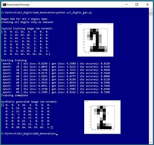
A good way to see where this article is headed is to take a look at the screenshot of a demo program in Figure 1. The demo generates synthetic images of handwritten "2" digits based on the UCI Digits dataset. Each image is 8 by 8 pixels with values between 0 and 16. The demo begins by loading 380 actual "2" digit images into memory. A typical "2" digit from the training data is displayed. Next, the demo trains a GAN model using the 380 images. The demo finishes by using the trained GAN to generate a synthetic "2 "image.

This article assumes you have an intermediate or better familiarity with a C-family programming language, preferably Python, and a basic familiarity with the PyTorch code library. The source code for the demo program is a bit too long to present in its entirety in this article, but the complete code and training data are available in the accompanying file download. The training data is embedded as comments in the source code.

GANs are complex, both conceptually and technically, so this article focuses on explaining the key ideas you need to understand so that you can create GANs to suit your problem scenarios. All normal error checking code has been omitted to keep the main ideas as clear as possible.

To run the demo program, you must have Python and PyTorch installed on your machine. The demo programs were developed on Windows 10 using the Anaconda 2020.02 64-bit distribution (which contains Python 3.7.6) and PyTorch version 1.8.0 for CPU installed via pip. Installation is not trivial. You can find detailed step-by-step installation instructions in my blog post.

The UCI Digits Dataset
The UCI Digits dataset can be found online. There is a 3,823-item file named optdigits.tra (intended for training) and a 1,797-item file named optdigits.tes (for testing). I downloaded the files and renamed them to optdigits_train_3823.txt and optdigits_test_1797.txt. Each file is a simple, comma-delimited text file. Each line represents an 8 by 8 handwritten digit from "0" to "9."

The UCI Digits data looks like:

0,1,6,16,12, . . . 1,0,0,13,0
2,7,8,11,15, . . . 16,0,7,4,1
. . .

The first 64 values on each line are the image pixel values. Each pixel is a grayscale value between 0 and 16. The last value on each line is the digit/label. There are about 380 of each digit in the training file and about 180 of each digit in the test file, but the digits are not evenly distributed. The counts of each "0" though "9" digit in the training data are: 376, 389, 380, 389, 387, 376, 377, 387, 380 and 382.

I wrote a short utility program to scan through the training data file and select out the 380 "2" digits and save them as file uci_digits_2_only.txt using the same comma-delimited format.

The demo program defines a PyTorch Dataset class to load the data into memory. See Listing 1.

Listing 1: A Dataset Class for the UCI Digits Data

import torch as T
import numpy as np

class UCI_Digits_Dataset(T.utils.data.Dataset):
  # like: 8,12,0,16, . . 15,7
  # 64 pixel values [0-16], digit [0-9]

  def __init__(self, src_file, n_rows=None):
    tmp_x = np.loadtxt(src_file, max_rows=n_rows,
      usecols=range(0,64), delimiter=",", comments="#",
      dtype=np.float32)  # just pixels, no labels
    tmp_x /= 16.0        # normalize
    self.x_data = T.tensor(tmp_x, 
      dtype=T.float32).to(device) 

  def __len__(self):
    return len(self.x_data)

  def __getitem__(self, idx):
    return self.x_data[idx]

The class loads a file of UCI digits data into memory as a two-dimensional array using the NumPy loadtxt() function. The pixel values are normalized to a range of 0.0 to 1.0 by dividing by 16, which is important for GAN architecture. The NumPy array is converted to a PyTorch tensor and items are served up one at a time by the __getitem__() function.

The Dataset can be called like this:

fn = ".\\Data\\ uci_digits_2_only.txt "
my_ds = UCI_Digits_Dataset(fn)
my_ldr = T.utils.data.DataLoader(my_ds, \
  batch_size=10, shuffle=True)
for (b_ix, batch) in enumerate(my_ldr):
  # b_ix is the batch index
  # batch has 10 items with 64 values between 0 and 1
. . .

The Dataset object is passed to a built-in PyTorch DataLoader object. The DataLoader object serves up the data in batches of a specified size, in a random order on each pass through the Dataset.

The design pattern presented here will work for most generative adversarial network scenarios. If your raw data contains a categorical variable, such as "color" with possible values "red", "blue" or "green," you can one-hot encode the data: "red" = (1, 0, 0), "blue" = (0, 1, 0), "green" = (0, 0, 1).

Understanding Generative Adversarial Networks
My explanation of generative adversarial networks will take some liberties with terminology and details to help make the explanation easier to understand. Briefly, a GAN is a system that has two interconnected deep neural networks. One network is called the Generator; the other network is called the Discriminator.

The Generator accepts random values and emits a synthetic data item. The ultimate goal of a GAN is to generate good synthetic data items.

The Discriminator is a helper network that's a binary classifier. The Discriminator accepts a data item, which can be either real (from the training data) or fake (from the Generator), and then emits a pseudo-probability value between 0 and 1 where a value less than 0.5 indicates a fake item and a value greater than 0.5 indicate a real item.

Expressed in high-level pseudo-code, one iteration of training a GAN (for image data) is:

fetch a batch of real images from training data
  feed real images to Discriminator, compute loss
  
  make a batch of fake images using Generator
  feed fake images to Discriminator, compute loss
  
  combine the two loss values
  use combined loss to update Discriminator
  
  make a batch of fake images using Generator
  feed fake images to Discriminator, compute reverse loss
  use reverse loss to update Generator

The training process alternates between updating the Discriminator, so that it can better detect fake images produced by the Generator, and updating the Generator so that it produces fake images that are more likely to fool the Discriminator. When training finishes, a good Generator will fool the Discriminator about half the time, which means the Discriminator cannot easily distinguish a fake image from a real image.

There are many possible architecture and design alternatives for a GAN. The design presented in this article is relatively simple and is based mostly on the original 2014 GAN research article "Generative Adversarial Networks" by I. Goodfellow et al.

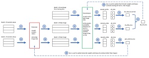
The diagram in Figure 2 shows the relationship between the Generator and the Discriminator, and one training iteration for the demo GAN. Your immediate reaction is probably something like, "That looks fairly complicated." You would be correct.

Steps 1 through 10 train the Discriminator binary classifier. A regular non-GAN binary classifier is trained using data that contains both class 0 and class 1 data items. In a GAN, the class 1 items are the real images from training data and the class 0 items are fake images from the Generator. The two loss values are computed separately and then combined by adding. An alternative design is to construct a batch of combined real and fake data, feed the combined data to the Discriminator, and compute a single loss value.

Steps 11 through 16 train the Generator. Suppose the Generator creates a batch of poor fake images (12). The Discriminator will easily identify the images as fake and the output (14) will be pseudo-probabilities close to 0. When compared against an all_ones tensor (15) the loss value will be large and the weights of the Generator neural network will be updated significantly, making the Generator better.

But suppose the Generator creates a batch of very good fake images. The Discriminator will think the images are real and so the pseudo-probabilities in (14) will be close to 1. When compared to an all_ones tensor, the loss will be very small and the weights of the Generator neural network will not change much. Clever!

Defining the GAN Generator
The code that defines the demo GAN Generator is presented in Listing 2. The architecture is 20-40-64 which means that the network accepts 20 random values, expands them to 40 intermediate values. Then the 40 values are expanded to 64 values between 0 and 1, where each is a normalized pixel.

Listing 2: GAN Generator Definition

class Generator(T.nn.Module):  # 20-40-64
  def __init__(self): 
    super(Generator, self).__init__()
    self.fc1 = T.nn.Linear(20, 40)
    self.fc2 = T.nn.Linear(40, 64)

    self.inpt_dim = 20

    T.nn.init.xavier_uniform_(self.fc1.weight)
    T.nn.init.zeros_(self.fc1.bias)
    T.nn.init.xavier_uniform_(self.fc2.weight)
    T.nn.init.zeros_(self.fc2.bias)

  def forward(self, x):      # 20
    z = T.tanh(self.fc1(x))  # 40
    oupt = T.sigmoid(self.fc2(z))  # 64
    return oupt

The output activation function is sigmoid() so that a generated fake image will have normalized pixel values between 0 and 1. The hidden layer activation is tanh(). One of the reasons why GANs are so complicated is that both the Generator and Discriminator have many hyperparameters such as number of hidden layers, activation function on hidden nodes, weight and bias initialization algorithm, and size of Generator input.

Defining the GAN Discriminator
The code that defines the demo GAN Discriminator binary classifier is presented in Listing 3. The architecture is 64-32-16-1 which means that the network accepts 64 values between 0 and 1 that represent either a real image or a fake image. The network has a single output node which, when used with binary cross entropy loss, is the usual design for a binary classifier.

Listing 3: GAN Discriminator Definition

class Discriminator(T.nn.Module):  # 64-32-16-1
  def __init__(self):
    super(Discriminator, self).__init__()
    self.fc1 = T.nn.Linear(64, 32)
    self.fc2 = T.nn.Linear(32, 16)
    self.fc3 = T.nn.Linear(16, 1)

    T.nn.init.xavier_uniform_(self.fc1.weight)
    T.nn.init.zeros_(self.fc1.bias)
    T.nn.init.xavier_uniform_(self.fc2.weight)
    T.nn.init.zeros_(self.fc2.bias)
    T.nn.init.xavier_uniform_(self.fc3.weight)
    T.nn.init.zeros_(self.fc3.bias)
        
  def forward(self, x):      # 64
    z = T.tanh(self.fc1(x))  # 32
    z = T.tanh(self.fc2(z))  # 16
    oupt = T.sigmoid(self.fc3(z))  # 1
    return oupt

To recap, when designing a GAN, the Generator will have an x-(y-y)-z architecture where the number of output nodes, z, equals the number of values in a data item. The output activation function is usually sigmoid(). The number of input nodes, x, is a hyperparameter. A general rule of thumb I use is to start by trying sqrt(z) or z/2 or z/4 for the number of input nodes. The number of hidden layers and the number of hidden nodes in each layer, y, and the hidden activation function are hyperparameters. A general rule of thumb for the number of hidden nodes is to try a value about halfway between the number of input nodes and the number of output nodes. I usually first try tanh() or relu() for hidden node activation.

The Discriminator will have a z-(w-w)-1 architecture. The number of input nodes, z, equals the number of values in a data item. The number of hidden layers, the number of nodes in each hidden layer, and the activation function on the hidden nodes, are hyperparameters. I often first try two hidden layers with about z/2 and z/4 nodes. I usually try tanh() or relu() hidden node activation. The Discriminator output node activation is usually sigmoid().

Overall Program Structure
The overall demo program structure, with a few minor edits to save space, is presented in Listing 4. The demo begins by importing the required core NumPy and Torch libraries. The matplotlib library is used to display images, so you won't need it if your data items aren't images.

Listing 4: Overall GAN Program Structure

# uci_digits_gan.py

# GAN to generate synthetic '2' digits
# PyTorch 1.8.0-CPU Anaconda3-2020.02 (Python 3.7.6)
# Windows 10 

import numpy as np
import torch as T
import matplotlib as mpl
import matplotlib.pyplot as plt

device = T.device("cpu") 

# -----------------------------------------------------------

class UCI_Digits_Dataset(T.utils.data.Dataset):
  # see Listing 1

class Generator(T.nn.Module):  # 20-40-64
  # see Listing 2

class Discriminator(T.nn.Module):  # 64-32-16-1
  # see Listing 3

# -----------------------------------------------------------

def accuracy(gen, dis, n, verbose=False): . . 

def display_digit(x, save=False): . . 

def main():
  # 0. get started
  print("Begin GAN for UCI 2 digits demo ")
  np.random.seed(0)
  T.manual_seed(0)
  np.set_printoptions(linewidth=36)
  mpl.rcParams['toolbar'] = 'None'

  # 1. create data objects
  print("Creating UCI Digits only-2s Dataset ")
  train_file = ".\\Data\\uci_digits_2_only.txt" 
  train_ds = UCI_Digits_Dataset(train_file)
  bat_size = 10
  train_ldr = T.utils.data.DataLoader(train_ds,
    batch_size=bat_size, shuffle=True, drop_last=True)  

  # 1b. show typical training item (item [5])
  print("Typical training image (de-normed): ")
  digit = np.rint(train_ds[5].numpy() * 16)
  print(digit)
  display_digit(train_ds[5], save=False)

  # 2. create networks
  dis = Discriminator().to(device)  # 64-32-16-1
  gen = Generator().to(device)      # 20-40-64

  # 3. train GAN model
  max_epochs = 100
  ep_log_interval = 10
  lrn_rate = 0.005

  dis.train()  # set mode
  gen.train()
  dis_optimizer = T.optim.Adam(dis.parameters(), lrn_rate)
  gen_optimizer = T.optim.Adam(gen.parameters(), lrn_rate)
  loss_func = T.nn.BCELoss()
  all_ones = T.ones(bat_size, dtype=T.float32).to(device)
  all_zeros = T.zeros(bat_size, dtype=T.float32).to(device)

  print("Starting training ")
  for epoch in range(0, max_epochs):
    for (batch_idx, real_images) in enumerate(train_ldr):
      dis_accum_loss = 0.0  # to display progress
      gen_accum_loss = 0.0

      # 3a. train discriminator using real images
      dis_optimizer.zero_grad()
      dis_real_oupt = dis(real_images).reshape(-1)  # [0, 1]
      dis_real_loss = loss_func(dis_real_oupt,
        all_ones)  # or use squeeze()

      # 3b. train discriminator using fake images
      zz = T.normal(0.0, 1.0,
        size=(bat_size, gen.inpt_dim)).to(device)  # 10 x 20
      fake_images = gen(zz)
      dis_fake_oupt = dis(fake_images).reshape(-1)
      dis_fake_loss = loss_func(dis_fake_oupt, all_zeros)     
      dis_loss_tot = dis_real_loss + dis_fake_loss
      dis_accum_loss += dis_loss_tot

      dis_loss_tot.backward()  # compute gradients
      dis_optimizer.step()     # update weights and biases

      # 3c. train gen with fake images
      gen_optimizer.zero_grad()
      zz = T.normal(0.0, 1.0,
        size=(bat_size, gen.inpt_dim)).to(device)  # 20
      fake_images = gen(zz)
      dis_fake_oupt = dis(fake_images).reshape(-1)
      gen_loss = loss_func(dis_fake_oupt, all_ones)
      gen_accum_loss += gen_loss

      gen_loss.backward()
      gen_optimizer.step()

    if epoch % ep_log_interval == 0:
      acc_dis = Accuracy(gen, dis, 500, verbose=False)
      print(" epoch: %4d | dis loss: %0.4f | gen loss: %0.4f \
| dis accuracy: %0.4f "\
        % (epoch, dis_accum_loss, gen_accum_loss, acc_dis))

  print("Training complete ")

# -----------------------------------------------------------

  # 4. TODO: save trained model

  # 5. use generator to make fake images
  gen.eval()   # set mode
  for i in range(1):  # just 1 image for demo
    rinpt = T.randn(1, gen.inpt_dim).to(device)  # wrap normal()
    with T.no_grad():
      fi = gen(rinpt).numpy()  # make image, convert to numpy
    fi = np.rint(fi * 16)

    print("\nSynthetic generated image (de-normed): ")
    print(fi) 
    display_digit(fi)

# -----------------------------------------------------------

if __name__ == "__main__":
  main()

For simplicity, most of the program control logic is defined in main() function. The program defines two helper functions, accuracy() and display_digit(). The accuracy() function generates n fake images using the Generator, with its current weights and biases, and then sends the fake images to the Discriminator where they are classified as real (p > 0.5) or fake (p < 0.5). Knowing when to stop training a GAN is tricky. The accuracy of the Discriminator will vary during training as the Generator and Discriminator takes turns gaining the upper hand, but Discriminator accuracy values that are close to 50 percent are good.

The main() function sets the NumPy and PyTorch random number seeds so that results are reproducible:

def main():
  # 0. get started
  print("Begin GAN for UCI 2 digits demo ")
  np.random.seed(0)
  T.manual_seed(0)
  np.set_printoptions(linewidth=36)
  mpl.rcParams['toolbar'] = 'None'

The seed values of 0 are arbitrary. The rcParams['toolbar'] statement suppresses the toolbar on the MatPlotLib display, just to make the image a bit smaller.

Next, the program sets up Dataset and DataLoader objects:

# 1. create data objects
print("Creating UCI Digits only-2s Dataset ")
train_file = ".\\Data\\uci_digits_2_only.txt" 
train_ds = UCI_Digits_Dataset(train_file)
bat_size = 10
train_ldr = T.utils.data.DataLoader(train_ds,
  batch_size=bat_size, shuffle=True, drop_last=True)

The drop_last argument isn't needed in the demo because there are 380 training images and the batch size is 10, so each batch will have 38 items. The batch size is a hyperparameter that must be determined by trial and error.

The GAN is composed of two separate neural networks:

# 2. create networks
dis = Discriminator().to(device)  # 64-32-16-1
gen = Generator().to(device)      # 20-40-64

An alternative design is to define an explicit GAN class that encapsulates the Generator and the Discriminator.

Training the GAN is prepared like so:

# 3. train GAN model
max_epochs = 100
ep_log_interval = 10
lrn_rate = 0.005
dis.train()
gen.train()
dis_optimizer = T.optim.Adam(dis.parameters(), lrn_rate)
gen_optimizer = T.optim.Adam(gen.parameters(), lrn_rate)
loss_func = T.nn.BCELoss()
all_ones = T.ones(bat_size, dtype=T.float32).to(device)
all_zeros = T.zeros(bat_size, dtype=T.float32).to(device)

GANs are notoriously difficult to train, in part because there are more training parameters than in a regular neural network. The demo uses Adam optimization which often, but not always, works better than SGD (stochastic gradient descent) when training a GAN.

Training begins by computing the Discriminator loss on real images from the training data:

print("Starting training ")
for epoch in range(0, max_epochs):
  for (batch_idx, real_images) in enumerate(train_ldr):
    dis_accum_loss = 0.0  # to display progress
    gen_accum_loss = 0.0

    # 3a. train discriminator using real images
    dis_optimizer.zero_grad()
    dis_real_oupt = dis(real_images).reshape(-1)  # [0, 1]
    dis_real_loss = loss_func(dis_real_oupt,
      all_ones)  # or use squeeze()

These statements correspond to steps 1 through 3 in Figure 2. The reshape(-1) function converts the output pseudo-probabilities, which are in a 2-dimensional tensor, to a 1-dimensional tensor. This is one of the tricky syntax issues that can cost you a lot of time when working with GANs. An alternative to reshape(-1) is squeeze(). The dis_accum_loss and gen_accum_loss variables are used only to display cumulative loss values during training so you can check for situations where training is completely failing.

Next, the Discriminator loss on fake images is computed, losses are combined, and the Discriminator is updated:

# 3b. train discriminator using fake images
zz = T.normal(0.0, 1.0,
  size=(bat_size, gen.inpt_dim)).to(device)  # 10 x 20
fake_images = gen(zz)
dis_fake_oupt = dis(fake_images).reshape(-1)
dis_fake_loss = loss_func(dis_fake_oupt, all_zeros)     
dis_loss_tot = dis_real_loss + dis_fake_loss
dis_accum_loss += dis_loss_tot
dis_loss_tot.backward()  # compute gradients
dis_optimizer.step()     # update weights and biases

These statements correspond to steps 4 through 10 in Figure 2. The input to the Discriminator is a batch (10 items) of 20 random values. The random values are generated using the torch.normal() function. Each value is Gaussian (Normal) distributed with mean = 0.0 and standard deviation = 1.0. An alternative is to use Uniform distributed values.

Next, the Generator is trained using fake images that it generates:

# 3c. train gen with fake images
gen_optimizer.zero_grad()
zz = T.normal(0.0, 1.0,
  size=(bat_size, gen.inpt_dim)).to(device)
fake_images = gen(zz)
dis_fake_oupt = dis(fake_images).reshape(-1)
gen_loss = loss_func(dis_fake_oupt, all_ones)
gen_accum_loss += gen_loss
gen_loss.backward()
gen_optimizer.step()

These statements correspond to steps 11 through 16 in Figure 2. This is the trickiest part of the GAN system. Output from the Discriminator is used to compute a sort of reverse loss which is then used to update the Generator.

During training, Generator loss, Discriminator loss and Discriminator classification accuracy are displayed every ep_log_interval = 10 epochs:

if epoch % ep_log_interval == 0:
  acc_dis = accuracy(gen, dis, 500, verbose=False)
  print(" epoch: %4d | dis loss: %0.4f | gen loss: %0.4f \
  | dis accuracy: %0.4f "\
      % (epoch, dis_accum_loss, gen_accum_loss, acc_dis))
print("Training complete ")

In a non-demo scenario, you might want to create a checkpoint to save the state of the system so that if training fails, you can recover without having to start from scratch.

The demo concludes by using the trained GAN to generate and display a synthetic "2" digit:

. . .
  # 5. use generator
  gen.eval()   # set mode
  for i in range(1):  # just 1 image for demo
    rinpt = T.randn(1, gen.inpt_dim).to(device)  # wrap normal()
    with T.no_grad():
      fi = gen(rinpt).numpy()  # make image, convert to numpy
    fi = np.rint(fi * 16)
    print("Synthetic generated image (de-normed): ")
    print(fi) 
    display_digit(fi)

if __name__ == "__main__":
  main()

The Generator is set into eval() mode. Technically this is not necessary because the Generator doesn't use dropout or batch normalization, but explicitly setting mode is good practice in my opinion.

The random input is generated using the torch.randn() function which is just a wrapper around the torch.normal() function that was used in the training code. The point of using randn() is to illustrate that when using PyTorch there are often several different functions available that do the same thing.

The Accuracy Function
Because the Generator and the Discriminator in a GAN are constantly trying to trick each other during training, the loss values for the two networks will jump around. In many situations, computing and monitoring the classification accuracy of the Discriminator is useful. If the Discriminator has close to 100 percent accuracy, that means the Generator isn't producing very good fake data items. If the Discriminator has close to 0 percent accuracy, that means the Discriminator hasn't been trained well. If the Discriminator has close to 50 percent accuracy, that can mean that the Generator is producing realistic data items.

The demo program defines a helper accuracy() function. The code is presented in Listing 5. The function uses the Generator to create a specified number (500 in the demo program) of fake data items, feeds those items to the Discriminator, which calculates how many of the fake items were corrected classified as fake.

Listing 5: An Accuracy Function for the Discriminator

def accuracy(gen, dis, n, verbose=False):
  gen.eval(); dis.eval()
  n_correct = 0; n_wrong = 0

  for i in range(n):
    zz = T.normal(0.0, 1.0,
      size=(1, gen.inpt_dim)).to(device)  # 20 values
    fake_image = gen(zz)  # one fake image
    pp = dis(fake_image)  # pseudo-prob
    if pp < 0.5:
      n_correct += 1      # discriminator knew it was fake
    else:
      n_wrong += 1        # dis thought it was a real image

    if verbose == True:
      print("")
      print(fake_image)
      print(pp)
      input()
  return (n_correct * 1.0) / (n_correct + n_wrong)

In pseudo-code, function accuracy() is:

loop n times
    make a fake image using Generator
    send fake image to Discriminator, get pseudo-prob
    if pseudo-prob < 0.5:
      num_correct += 1 # Discriminator knew item was fake
    else
      num_wrong += 1  # Discriminator thought item was real
  end-loop
  return num_correct / (num_correct + num_wrong)

The accuracy function iterates one fake data item at a time. This is approach is slow but allows you to pause program execution and investigate items. Performance is rarely an issue when working with GANs, but if speed is necessary you can refactor accuracy() to construct all fake items at the same time using normal() and then compute all accuracies at the same time.

Wrapping Up
Generative adversarial networks produced a lot of interest in the research and engineering communities when they were first introduced in 2014. Since then, enthusiasm in the research community has remained high, but enthusiasm in the engineering community has waned a bit. I suspect that there are several reasons for the decline in enthusiasm for GANs. From an engineering perspective, GANs are very difficult to train. From a pragmatic perspective, it's difficult to measure how good GAN-created fake data items are.

Researchers have produced dozens of variations of GANs, sometimes referred to as the GAN Zoo. These variations include Info GAN, Conditional GAN, Cycle GAN, f-GAN, Wasserstein GAN and many others. Because publish-or-perish is a very real phenomenon in research, it's not entirely clear how much of research enthusiasm for GANs is due to the subject's complexity which encourages a vast number of exploration paths, and how much enthusiasm is due to a search for practical applications of GANs. Many deep neural architectures turned out to have unexpected and surprising applications, and this could be true of GANs too.

• Get Code Download