The Data Science Lab
Computing the Similarity Between Two Machine Learning Datasets
At first thought, computing the similarity/distance between two datasets sounds easy, but in fact the problem is extremely difficult, explains Dr. James McCaffrey of Microsoft Research.
A fairly common sub-problem in many machine learning and data science scenarios is the need to compute the similarity (or difference or distance) between two datasets. For example, if you select a sample from a huge set of training data, you likely want to know how similar the sample dataset is to the source dataset. Or if you want to prime the training for a very deep neural network, you need to find an existing model that was trained using a dataset that is most similar to your new dataset.
At first thought, computing the similarity/distance between two datasets sounds easy, but in fact the problem is extremely difficult. If you try to compare individual lines between datasets, you quickly run into the combinatorial explosion problem -- there are just too many comparisons. There are also the related problems of dealing with different dataset sizes, and dealing with non-numeric data. The bottom line is that in most scenarios there's no simple way to calculate the distance between two datasets.
This article explains how to compute the distance between any two datasets using a combination of neural and classical statistics techniques. A good way to see where this article is headed is to take a look at the screenshot of a demo program in Figure 1.
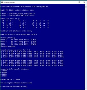 [Click on image for larger view.] Figure 1: UCI Digits Dataset Distance Demo Run
The goal of the demo is to compute the distance between a dataset P, which is 100 lines from the UCI Digits dataset, and a dataset Q, which is the same as the P dataset but with 50 percent of the lines of data randomized. The computed distance between the two datasets is 1.6625. Larger values of dataset distance indicate greater dissimilarity.
Each line of data in the P and Q datasets represents an 8x8 handwritten digit. Each line has 65 numbers. The first 64 numbers are greyscale pixel values from 0 to 16. The last number is the associated digit label, from 0 to 9. The demo loads the P and Q data into memory and then trains a 65-32-4-32-65 deep neural autoencoder using the P dataset. The result is an autoencoder than converts each image (and its label) into a vector of four values where each value is a number between 0.0 and 1.0.
Next, the demo takes each image item in P and Q and uses the autoencoder to convert them to a 4-valued vector. Then, each of the four components of the two datasets are binned into 10 frequency buckets. The last step is to compute the four distances between the four pairs of frequency distributions, which gives (2.18, 1.06, 2.68, 0.73). The four distances are averaged to give the final distance of 1.6625 between P and Q. The process is much simpler than it sounds.
This article assumes you have an intermediate or better familiarity with a C-family programming language, preferably Python, and a basic familiarity with the PyTorch code library. The complete source code for the demo program is presented in this article, and the complete code is also available in the accompanying download. The data for the two data files used in the demo program are embedded as comments at the end of the source code download file.
To run the demo program, you must have Python and PyTorch installed on your machine. The demo programs were developed on Windows 10 using the Anaconda 2020.02 64-bit distribution (which contains Python 3.7.6) and PyTorch version 1.8.0 for CPU installed via pip. Installation is not trivial. You can find detailed step-by-step installation instructions in my blog post.
The Autoencoder Component
The autoencoder definition for the demo program is presented in Listing 1. The architecture is 65-32-4-32-65. The input has 65 nodes, one for each input in the UCI Digits dataset. The latent dimension is a hyperparameter and is set to 4. You can think of the latent dimension as the number of abstract attributes that represent a data item. For example, each image of a digit might be represented by "roundness," "sharpness," "thickness" and "lateral-ness."
Listing 1: The Autoencoder Definition
import numpy as np
import torch as T
device = T.device("cpu")

class Autoencoder(T.nn.Module):  # 65-32-4-32-65
  def __init__(self):
    super(Autoencoder, self).__init__()
    self.layer1 = T.nn.Linear(65, 32)  # includes labels
    self.layer2 = T.nn.Linear(32, 4)
    self.layer3 = T.nn.Linear(4, 32)
    self.layer4 = T.nn.Linear(32, 65)
    self.latent_dim = 4

  def encode(self, x):
    z = T.tanh(self.layer1(x))
    z = T.sigmoid(self.layer2(z))
    return z

  def decode(self, x):
    z = T.tanh(self.layer3(x))
    z = T.sigmoid(self.layer4(z))
    return z

  def forward(self, x):
    z = self.encode(x)
    oupt = self.decode(z)
    return oupt
The encode() method applies sigmoid activation on the latent layer so that all values will be in the range [0.0, 1.0]. This allows frequency distributions to be easily computed. The decode() method also uses sigmoid activation, on the output layer. This means that input data must be normalized to a range of [0.0, 1.0] so that input can be directly compared to output. Therefore, the 64 input pixel values, which are all between 0 and 16, must be divided by 16. The class labels, which are between 0 and 9, must be divided by 9.
The program-defined train() function is presented in Listing 2. The train() function accepts a PyTorch Dataset object. The train() function uses Adam optimization with a hard-coded learning rate set to 0.001. You might want to parameterize the learning rate to make it a bit easier to experiment to find a good value for your particular problem scenario.
Listing 2: Training the Autoencoder
def train(ae, ds, bs, me, le):
  # train autoencoder ae with dataset ds using batch
  # size bs, with max epochs me, log_every le
  data_ldr = T.utils.data.DataLoader(ds, \
    batch_size=bs, shuffle=True)

  loss_func = T.nn.MSELoss()
  opt = T.optim.Adam(ae.parameters(), lr=0.001)
  print("Starting training")
  for epoch in range(0, me):
    for (b_idx, batch) in enumerate(data_ldr):
      opt.zero_grad()
      X = batch
      oupt = ae(X)
      loss_val = loss_func(oupt, X)  # note X not Y
      loss_val.backward()
      opt.step()

    if epoch > 0 and epoch % le == 0:
      print("epoch = %6d" % epoch, end="")
      print("  curr batch loss = %7.4f" % \
        loss_val.item(), end="")
      print("")
  print("Training complete ")
The Dataset definition is presented in Listing 3. Notice that the 64 pixel values and the class label are programmatically normalized to a [0.0, 1.0] range. If your data has categorical variables, such as color with possible values (red, blue, green), you can use one-hot encoding: red = (1, 0, 0), blue = (0, 1, 0), green = (0, 0, 1). By using one-hot encoding you simultaneously solve the problems of non-numeric data and normalization. If your data has Boolean data, you should encode it using 0-1 encoding rather than minus-one-plus-one encoding.
Listing 3: Dataset Definition
class Digits_Dataset(T.utils.data.Dataset):
  # for an Autoencoder (not a classifier)
  # assumes data is:
  # 64 pixel values (0-16) (comma) label (0-9)
  # [0] [1] . . [63] [64]

  def __init__(self, src_file):
    all_xy = np.loadtxt(src_file, usecols=range(65),
      delimiter=",", comments="#", dtype=np.float32)
    self.xy_data = T.tensor(all_xy, dtype=T.float32).to(device)
    self.xy_data[:, 0:64] /= 16.0  # normalize pixels
    self.xy_data[:, 64] /= 9.0     # normalize labels

  def __len__(self):
    return len(self.xy_data)

  def __getitem__(self, idx):
    xy = self.xy_data[idx]
    return xy
Converting the Data to Frequency Distributions
The autoencoder component converts each data item to a vector of four latent values, such as [0.54, 0.93, 0.11, 0.63]. Each of the four latent values generates a frequency distribution. The work is done by program-defined function make_freq_mat() and a helper value_to_bin() function. These two functions are presented in Listing 4.
Listing 4: Functions to Construct Frequency Distributions
def value_to_bin(x):
  # x is in [0.0, 1.0]
  if x >= 0.0 and x < 0.1:   return 0
  elif x >= 0.1 and x < 0.2: return 1
  elif x >= 0.2 and x < 0.3: return 2
  elif x >= 0.3 and x < 0.4: return 3
  elif x >= 0.4 and x < 0.5: return 4
  elif x >= 0.5 and x < 0.6: return 5
  elif x >= 0.6 and x < 0.7: return 6
  elif x >= 0.7 and x < 0.8: return 7
  elif x >= 0.8 and x < 0.9: return 8
  else:                      return 9

# -----------------------------------------

def make_freq_mat(ae, ds):
  d = ae.latent_dim
  result = np.zeros((d,10), dtype=np.int64)
  n = len(ds)
  for i in range(n):
    x = ds[i]
    with T.no_grad():
      latents = ae.encode(x)
    latents = latents.numpy()
    for j in range(d):
      bin = value_to_bin(latents[j])
      result[j][bin] += 1
  result = (result * 1.0) / n
  return result
The code is quite simple, but the idea is a bit tricky. Suppose the latent dimension is just two (instead of four as in the demo) and you have just eight data items (instead of 100). Each data item gives a vector with two values. Suppose they are:
(0.23, 0.67)
(0.93, 0.55)
(0.11, 0.38)
(0.28, 0.72)
(0.53, 0.83)
(0.39, 0.21)
(0.84, 0.79)
(0.22, 0.61)
The first frequency distribution looks at just the first values: (0.23, 0.93, 0.11, 0.28, 0.53, 0.39, 0.84, 0.22). If there are 10 bins, the bins are [0.0 to 0.1), [0.1 to 0.2), . . . [0.9 to 1.0]. The bin counts for the first latent dim are: (0, 1, 3, 1, 0, 1, 0, 0, 1, 1). Because there are eight items, the frequency distribution is (0.000, 0.125, 0.375, 0.125, 0.000, 0.125, 0.000, 0.000, 0.125, 0.125).
Similarly, the counts for the second latent dim are (0, 0, 1, 1, 0, 1, 2, 2, 1, 0) and the frequency distribution is (0.000, 0.000, 0.125, 0.125, 0.000, 0.125, 0.250, 0.250, 0.125, 0.000).
Comparing the Frequency Distributions
There are several ways to compute the distance between two frequency distributions. Common distance functions include Kullback-Leibler divergence, Jensen-Shannon distance and Hellinger distance. The demo program uses a highly simplified version of the Wasserstein distance function called information transfer distance. Briefly, information transfer distance is the minimum amount of work required to transform one frequency distribution into another.
The distance measure is implemented as program-defined function info_transfer_distance() and two helper functions, move_info() and first_nonzero(). The implementations are presented in Listing 5.
Listing 5: The Information Transfer Distance Functions
def first_nonzero(vec):
  dim = len(vec)
  for i in range(dim):
    if vec[i] > 0.0:
      return i
  return -1  # no empty cells found

def move_info(src, si, dest, di):
  # move as much src at [si] as possible to dest[di]
  if src[si] <= dest[di]:     # move all in src
    mass = src[si]
    src[si] = 0.0             # all src got moved
    dest[di] -= mass          # less to fill now
  elif src[si] > dest[di]:    # use just part of src
    mass = dest[di]           # fill remainder of dest
    src[si] -= mass           # less info left in src
    dest[di] = 0.0            # dest is filled
  dist = np.abs(si - di)
  return mass * dist          # weighted info transfer

def info_transfer_distance(p, q):
  # distance between two p-dists p, q
  # highly simplified Wasserstein distance
  source = np.copy(p)
  destination = np.copy(q)
  tot_info = 0.0

  while True:  # TODO: add sanity counter check
    from_idx = first_nonzero(source)
    to_idx = first_nonzero(destination)
    if from_idx == -1 or to_idx == -1:
      break
    info = move_info(source, from_idx, \
      destination, to_idx)
    tot_info += info
  return tot_info
You can think of the info_transfer_distance() as a black box because it doesn't change regardless of the data. If two frequency distributions P and Q are the same, info_transfer_distance(P, Q) = 0. The greater the difference between P and Q, the larger the value of the function is. If frequencies are binned into 10 buckets, the maximum value of the information transfer distance function is 9.0.
Putting it All Together
The demo program begins by specifying the file names that hold the two datasets to be compared:
def main():
  # 0. get started
  print("Begin UCI Digits dataset distance demo ")
  T.manual_seed(1)
  np.random.seed(1)
  p_file = ".\\Data\\uci_digits_train_100.txt"
  q_file = ".\\Data\\digits_100_noise_50.txt"
. . .
The P file contains 100 randomly selected lines of the UCI Digits dataset. The Q file is the same as P but 50 percent of the lines were replaced by random values -- 0 to 16 for the 64 pixels and 0 to 9 for the class label.
Next, the two datasets are loaded into memory:
  print("P file = " + str(p_file))
  print("Q file = " + str(q_file))
  print("First five lines of Q: ")
  show_uci_file(q_file, 5)

  # 1. create Dataset objects
  print("Loading P and Q Datasets into memory ")
  p_ds = Digits_Dataset(p_file)
  q_ds = Digits_Dataset(q_file)
The show_uci_file() is program-defined and not really needed to compute dataset similarity. A simple print() statement would work fine. Next, an autoencoder is created and trained on the P reference dataset:
  # 2. create and train autoencoder model using parent
  print("Creating 65-32-4-32-65 autoencoder using P ")
  autoenc = Autoencoder()   # 65-32-4-32-65
  autoenc.train()           # set mode
  bat_size = 10
  max_epochs = 100
  log_every = 20
  train(autoenc, p_ds, bat_size, max_epochs,
    log_every)
The batch size and maximum number of training epochs are hyperparameters that must be tuned for each particular problem. Next, the four frequency distributions are computed:
  # 4. create frequency matrices for reference P and other Q
  print("Creating frequency arrays for P, Q ")
  p_freq = make_freq_mat(autoenc, p_ds)
  q_freq = make_freq_mat(autoenc, q_ds)
  np.set_printoptions(formatter={'float': '{: 0.3f}'.format})
  print(p_freq)
  print("")
  print(q_freq)
The demo concludes by computing the four information transfer distances between frequency distributions, and averaging them to give the final distance result:
. . .
  # 5. compute information transfer distances)
  print("Computing info transfer distances ")
  sum = 0.0
  for j in range(4):  # one distance for each pair latents
    dist = info_transfer_distance(p_freq[j], q_freq[j])
    print("%0.5f" % dist)
    sum += dist
  avg_dist = sum / 4
  print("Distance(P,Q) = %0.4f " % avg_dist)
if __name__ == "__main__":
  main()
You might want to wrap the entire main program logic into a class or a single high-level function. A wrapper function signature might look something like dataset_similarity(p_file, q_file, ae_ld, ae_bs, ae_me) where ae_ld is the autoencoder latent dimension size, ae_bs is the autoencoder training batch size, and ae_me is the maximum epochs used for training.
Testing the Dataset Distance Function
The dataset similarity / distance technique was tested by computing the distance between a dataset P and 10 other datasets that increased in difference from P. The P dataset is 100 randomly selected items from the UCI Digits dataset. The 10 Q datasets were constructed from P by replacing 10 percent, 20 percent, 30 percent, . . 100 percent of the lines in P with random values.
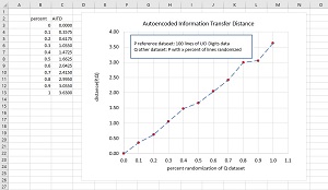 [Click on image for larger view.] Figure 2: Testing the Behavior of the Dataset Distance System
The idea is that as the randomness in Q increases, the dataset distance between P and Q should increase. The graph in Figure 2 shows that this is exactly what happens.
Wrapping Up
In informal usage, the term "metric" means anything that can be measured using a number. An example is the height of a person. But in the context of dataset similarity, "metric" has a very specific meaning. A formal distance metric is a function that satisfies three requirements. If p, q and r are three datasets, then a formal metric function dist(p, q) is one where:
- if p == q then dist(p, q) = 0, and if dist(p, q) = 0, p must equal q. [identity]
- dist(p, q) = dist(q, p). [symmetry]
- dist(p, q) <= dist(p, r) + dist(r, q). [triangle inequality]
The dataset similarity technique presented in this article is not a formal metric because dist(p, q) does not necessarily equal dist(q, p). This is because the autoencoder is trained using only the p dataset, and therefore p acts as a reference dataset relative to q. To make the technique presented in this article symmetric, you could write a wrapper function that returns the average of the distances when p is used as the reference dataset and when q is used as the reference.