The Data Science Lab
Naive Bayes Classification Using C#
Dr. James McCaffrey of Microsoft Research presents a full step-by-step example with all code to predict a person's optimism score from their occupation, eye color and country.
The goal of a naive Bayes classification problem is to predict a discrete value called the class label. The idea is best explained by a concrete example. Suppose you have a set of 40 data items where each item consists of a person's occupation (actor, baker, clerk or diver), eye color (green or hazel), country (Italy, Japan or Korea), and their personality optimism score (0, 1 or 2). You want to predict a person's optimism score from their occupation, eye color and country. This is an example of multiclass classification because the variable to predict, optimism, has three or more possible values. If the variable to predict has just two possible values, the problem would be called binary classification. Unlike some machine learning techniques, Naive Bayes can handle both multiclass and binary classification problems.
 [Click on image for larger view.]Figure 1: Naive Bayes Classification Using C# in Action
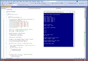
A good way to see where this article is headed is to take a look at the screenshot of a demo program in Figure 1. The demo sets up 40 data items -- occupation, eye-color, country, optimism. The first few data items are:
actor  green  korea  1
baker  green  italy  0
diver  hazel  japan  0
diver  green  japan  1
clerk  hazel  japan  2
Notice that all the data values are categorical (non-numeric). This is a key characteristic of the naive Bayes classification technique presented in this article . If you have numeric data, such as a person's age in years, you can bin the data into categories such as child, teen, adult.
The demo sets up an item to predict as ("baker", "hazel", "italy"). Next, the demo scans through the data and computes and displays smoothed ("add 1") joint counts. For example, the 5 in the screenshot means that there are 4 bakers who have optimism class = 0.
The demo computes the raw, unsmoothed class counts as (19, 14, 7). This means there are 19 people with optimism class = 0, 14 people with class = 1, and 7 people with class = 2. Notice that 19 + 14 + 7 = 40, the number of data items.
The smoothed joint counts and the raw class counts are combined mathematically to produce evidence terms of (0.0027, 0.0013, 0.0021). These correspond to the likelihoods of class (0, 1, 2). Because the largest evidence value is at index [0], the prediction for the ("baker", "hazel", "italy") person is class 0.
Evidence terms are somewhat difficult to interpret so the demo converts the three evidence terms to pseudo-probabilities: (0.4418, 0.2116, 0.3466). The values are not true mathematical probabilities but because they sum to 1.0 they can loosely be interpreted as probabilities. The largest probability is at index [0].
This article assumes you have intermediate or better programming skill with C-family language such as Python or Java, but doesn't assume you know anything about naive Bayes classification. The complete demo code and the associated data are presented in this article. The source code and the data are also available in the accompanying download. All normal error checking has been removed to keep the main ideas as clear as possible.
Understanding Naive Bayes Classification
The first step in naive Bayes classification is to compute the joint counts associated with the data item to predict. For ("baker", "hazel", "italy") and the 40-item demo data, the joint counts are:
baker and class 0 = 4
baker and class 1 = 0
baker and class 2 = 1
hazel and class 0 = 5
hazel and class 1 = 2
hazel and class 2 = 2
italy and class 0 = 1
italy and class 1 = 5
italy and class 2 = 1
The joint counts are multiplied together when computing the evidence terms. If any joint count is 0, the entire term is zeroed out, therefore 1 is added to each joint count to prevent this. This is called Laplacian smoothing.
The next step in naive Bayes classification is to compute the counts of each of the classes to predict. For the demo data the class counts are (19, 14, 7). It's not necessary to smooth the class counts because there will always be at least one of each class.
Next, an evidence term (sometimes called Z) is computed for each possible class value. For class 0, the evidence term is:
Z(0) = (5 / 19+3) * (6 / 19+3) * (2 / 19+3) * (19 / 40)
     = 4/22 * 5/22 * 1/22 * 19/40
     = 0.1818 * 0.2273 * 0.0435 * 0.4750
     = 0.0027
The last term, 19/40, is the probability of class 0. In the first three terms, the numerator is a smoothed joint count. The denominator is the raw class count with 3 (number of predictor values) added to compensate for the smoothing.
For class 1, the evidence term is:
Z(1) = (1 / 14+3) * (3 / 14+3) * (6 / 14+3) * (14 / 40)
     = 1/17 * 3/17 * 6/17 * 14/40
     = 0.0588 * 0.1765 * 0.3529 * 0.3500
     = 0.0013
And for class 2, the evidence term is:
Z(2) = (2 / 7+3) * (3 / 7+3) * (2 / 7+3) * (7 / 40)
     = 2/10 * 3/10 * 2/10 * 7/40
     = 0.2000 * 0.3000 * 0.2000 * 0.1750
     = 0.0021
The largest evidence term is associated with class 0 so that's the predicted class. To make the evidence terms easier to compare, they are often normalized so that they sum to 1.0. The sum of the evidence terms is 0.0027 + 0.0013 + 0.0021 = 0.0061. The normalized (pseudo-probabilities) are:
P(class 0) = 0.0027 / 0.0061 = 0.4418
P(class 1) = 0.0013 / 0.0061 = 0.2116
P(class 2) = 0.0021 / 0.0061 = 0.3466
Because each evidence term is the product of values that are less than 1, there's a chance that the calculation could run into trouble. Therefore, in practice, the computation of evidence terms uses the math log() of each value which allows additions and subtractions instead of multiplications and divisions.
The Demo Program
The complete demo program, with a few minor edits to save space, is presented in Listing 1. To create the program, I launched Visual Studio and created a new C# .NET Core console application named NaiveBayes. I used Visual Studio 2019 (free Community Edition), but the demo has no significant dependencies so any version of Visual Studio will work fine. You can use the Visual Studio Code program too.
After the template code loaded, in the editor window I removed all unneeded namespace references, leaving just the reference to the top-level System namespace. In the Solution Explorer window, I right-clicked on file Program.cs, renamed it to the more descriptive NaiveBayesProgram.cs, and allowed Visual Studio to automatically rename class Program to NaiveBayesProgram.
Listing 1: Complete Naive Bayes Demo Code
using System;
namespace NaiveBayes
{
  class NaiveBayesProgram
  {
    static void Main(string[] args)
    {
      Console.WriteLine("\nBegin naive Bayes classification ");
      string[][] data = GetData();
      Console.WriteLine("\nData looks like: ");
      Console.WriteLine("actor  green  korea  1");
      Console.WriteLine("baker  green  italy  0");
      Console.WriteLine("diver  hazel  japan  0");
      Console.WriteLine("diver  green  japan  1");
      Console.WriteLine("clerk  hazel  japan  2");
      Console.WriteLine(" . . . ");

      int nx = 3;  // number predictors (job, eye, country)
      int nc = 3;  // number classes (0, 1, 2)
      int N = 40;  // number data items

      int[][] jointCounts = new int[nx][];
      for (int i = 0; i < nx; ++i)
        jointCounts[i] = new int[nc];

      int[] yCounts = new int[nc];

      string[] X = new string[] { "baker", "hazel", "italy"};
      Console.WriteLine("\nItem to classify: ");
      Console.WriteLine("baker  hazel  italy");

      for (int i = 0; i < N; ++i) {   // compute joint counts
        int y = int.Parse(data[i][nx]);  // get the class as int
        ++yCounts[y];
        for (int j = 0; j < nx; ++j) {
          if (data[i][j] == X[j])
            ++jointCounts[j][y];
        }
      }

      for (int i = 0; i < nx; ++i)  // Laplacian smoothing
        for (int j = 0; j < nc; ++j)
          ++jointCounts[i][j];

      Console.WriteLine("\nJoint counts (smoothed): ");
      Console.WriteLine("0 1 2 ");
      Console.WriteLine("------");
      ShowMatrix(jointCounts);

      Console.WriteLine("\nClass counts (raw): ");
      ShowVector(yCounts);

      // compute evidence terms
      double[] eTerms = new double[nc];
      for (int k = 0; k < nc; ++k)
      {
        double v = 1.0;  // direct approach
        for (int j = 0; j < nx; ++j)
          v *= (jointCounts[j][k] * 1.0) / (yCounts[k] + nx);
        v *= (yCounts[k] * 1.0) / N;
        eTerms[k] = v;

        //double v = 0.0;  // use logs to avoid underflow
        //for (int j = 0; j < nx; ++j)
        //  v += Math.Log(jointCounts[j][k]) - Math.Log(yCounts[k] + nx);
        //v += Math.Log(yCounts[k]) - Math.Log(N);
        //eTerms[k] = Math.Exp(v);
      }

      Console.WriteLine("\nEvidence terms for each class: ");
      ShowVector(eTerms);

      double evidence = 0.0;
      for (int k = 0; k < nc; ++k)
        evidence += eTerms[k];

      double[] probs = new double[nc];
      for (int k = 0; k < nc; ++k)
        probs[k] = eTerms[k] / evidence;

      Console.WriteLine("\nPseudo-probabilities each class: ");
      ShowVector(probs);

      Console.WriteLine("\nEnd naive Bayes demo ");
      Console.ReadLine();
    } // Main

    static void ShowMatrix(int[][] m)
    {
      int r = m.Length; int c = m[0].Length;
      for (int i = 0; i < r; ++i)  {
        for (int j = 0; j < c; ++j)  {
          Console.Write(m[i][j] + " ");
        }
        Console.WriteLine("");
      }
    }

    static void ShowVector(int[] v)
    {
      for (int i = 0; i < v.Length; ++i)
        Console.Write(v[i] + "  ");
      Console.WriteLine("");
    }

    static void ShowVector(double[] v)
    {
      for (int i = 0; i < v.Length; ++i)
        Console.Write(v[i].ToString("F4") + "  ");
      Console.WriteLine("");
    }

    static string[][] GetData()
    {
      string[][] m = new string[40][];  // 40 rows
      m[0] = new string[] { "actor", "green", "korea", "1" };
      m[1] = new string[] { "baker", "green", "italy", "0" };
      m[2] = new string[] { "diver", "hazel", "japan", "0" };
      m[3] = new string[] { "diver", "green", "japan", "1" };
      m[4] = new string[] { "clerk", "hazel", "japan", "2" };
      m[5] = new string[] { "actor", "green", "japan", "1" };
      m[6] = new string[] { "actor", "green", "japan", "0" };
      m[7] = new string[] { "clerk", "green", "italy", "1" };
      m[8] = new string[] { "clerk", "green", "italy", "2" };
      m[9] = new string[] { "diver", "green", "japan", "1" };
      m[10] = new string[] { "diver", "green", "japan", "0" };
      m[11] = new string[] { "diver", "green", "japan", "1" };
      m[12] = new string[] { "diver", "green", "japan", "2" };
      m[13] = new string[] { "clerk", "green", "italy", "1" };
      m[14] = new string[] { "diver", "green", "japan", "1" };
      m[15] = new string[] { "diver", "hazel", "japan", "0" };
      m[16] = new string[] { "clerk", "green", "korea", "1" };
      m[17] = new string[] { "baker", "green", "japan", "0" };
      m[18] = new string[] { "actor", "green", "italy", "1" };
      m[19] = new string[] { "actor", "green", "italy", "1" };
      m[20] = new string[] { "diver", "green", "korea", "0" };
      m[21] = new string[] { "baker", "green", "japan", "2" };
      m[22] = new string[] { "diver", "green", "japan", "0" };
      m[23] = new string[] { "baker", "green", "korea", "0" };
      m[24] = new string[] { "diver", "green", "japan", "0" };
      m[25] = new string[] { "actor", "hazel", "italy", "1" };
      m[26] = new string[] { "diver", "hazel", "japan", "0" };
      m[27] = new string[] { "diver", "green", "japan", "2" };
      m[28] = new string[] { "diver", "green", "japan", "0" };
      m[29] = new string[] { "clerk", "hazel", "japan", "2" };
      m[30] = new string[] { "diver", "green", "korea", "0" };
      m[31] = new string[] { "diver", "hazel", "korea", "0" };
      m[32] = new string[] { "diver", "green", "japan", "0" };
      m[33] = new string[] { "diver", "green", "japan", "2" };
      m[34] = new string[] { "diver", "hazel", "japan", "0" };
      m[35] = new string[] { "actor", "hazel", "japan", "1" };
      m[36] = new string[] { "actor", "green", "japan", "0" };
      m[37] = new string[] { "actor", "green", "japan", "1" };
      m[38] = new string[] { "diver", "green", "japan", "0" };
      m[39] = new string[] { "baker", "green", "japan", "0" };
      return m;
    } // GetData()

  } // Program
} // ns
The demo program hard-codes the data inside a program-defined function GetData(). The data is returned as an array-of-arrays style matrix where each cell holds a string value. In a non-demo scenario you might want to store data in a text file and write a helper function to read the data into an array-of-arrays string[ ][ ] matrix.
All the control logic is in the Main() method. The key data structures are an array-of-arrays style int[ ][ ] matrix to hold the joint counts and an int[ ] vector to hold the class counts:
int nx = 3;  // number predictors (job, eye, country)
int nc = 3;  // number classes (0, 1, 2)
int N = 40;  // number data items

int[][] jointCounts = new int[nx][];
for (int i = 0; i < nx; ++i)
  jointCounts[i] = new int[nc];
int[] yCounts = new int[nc];
The raw class counts and the raw joint counts are computed like so:
string[] X = new string[] { "baker", "hazel", "italy"};
for (int i = 0; i < N; ++i) {   // compute joint counts
  int y = int.Parse(data[i][nx]);  // get the class as int
  ++yCounts[y];
  for (int j = 0; j < nx; ++j) {
    if (data[i][j] == X[j])
      ++jointCounts[j][y];
  }
}
The code walks through the data matrix row-by-row. The row class label is fetched as an int from the last value in the row at index [nx]. The class is used to increment the yCounts vector. Then the code walks through each predictor value and if the predictor value in the data matrix matches the predictor value in the item to predict, the corresponding entry in the jointCount matrix is incremented. After all joint count values have been computed, the demo code iterates through the matrix and adds 1 to each count so that there are no 0 values.
The evidence terms are computed by these statements:
double[] eTerms = new double[nc];
for (int k = 0; k < nc; ++k) {  // each class
  double v = 1.0;  // direct approach
  for (int j = 0; j < nx; ++j)
    v *= (jointCounts[j][k] * 1.0) / (yCounts[k] + nx);
  v *= (yCounts[k] * 1.0) / N;
  eTerms[k] = v;
}
If you want to avoid the possibility of numeric underflow, you can use this code:
double[] eTerms = new double[nc];
for (int k = 0; k < nc; ++k) {  // each class
  double v = 0.0;  // direct approach
  for (int j = 0; j < nx; ++j)
    v += Math.Log(jointCounts[j][k]) - Math.Log(yCounts[k] + nx);
  v += Math.Log(yCounts[k]) - Math.Log(N);
  eTerms[k] = Math.Exp(v);
}
The demo program concludes by normalizing the evidence terms so that they sum to 1.0 and can be loosely interpreted as probabilities. The pseudo-probabilities are displayed and the user can interpret the predicted class by finding the index of largest probability. If the predicted class (0, 1 or 2) needs to be passed to another system, you can programmatically compute the prediction by implementing a program-defined function (often called argmax() in languages such as Python).
Wrapping Up
Naive Bayes classification is called "naive" because it analyzes each predictor column independently. This doesn't take into account interactions between predictor values. For example, in the demo data, maybe clerks who have green eyes might have some special characteristics. The technique is "Bayesian" because the math is based on observed counts of data rather than some underlying theory.
The technique presented in this article works only with categorical data. There are other forms of naive Bayes classification that can handle numeric data. However, you must make assumptions about the math properties of the data, for example that the data has a normal (Gaussian) distribution with a certain mean and standard deviation.
Naive Bayes classification isn't used as much as it used to be because techniques based on neural networks are much more powerful. However, neural techniques usually require lots of data. Naive Bayes classification often works well with small datasets.