The Data Science Lab
Binary Classification Using New PyTorch Best Practices, Part 2: Training, Accuracy, Predictions
Dr. James McCaffrey of Microsoft Research explains how to train a network, compute its accuracy, use it to make predictions and save it for use by other programs.
This is the second of two articles that explain how to create and use a PyTorch binary classifier. A good way to see where this article is headed is to examine the screenshot of a demo program in Figure 1.
The demo program predicts the gender (male, female) of a person. The first article in the series explained how to prepare the training and test data, and how to define the neural network classifier. This article explains how to train the network, compute the accuracy of the trained network, use the network to make predictions and save the network for use by other programs.
A good way to see where this article is headed is to take a look at the screenshot of a demo program in Figure 1. The demo begins by loading a 200-item file of training data and a 40-item set of test data. Each tab-delimited line represents a person. The fields are gender (male = 0, female = 1), age, state of residence, annual income and politics type. The goal is to predict gender from age, state, income and politics type.
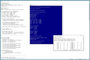 [Click on image for larger view.] Figure 1: Binary Classification Using PyTorch Demo Run
After the training data is loaded into memory, the demo creates an 8-(10-10)-1 neural network. This means there are eight input nodes, two hidden neural layers with 10 nodes each and one output node.
The demo prepares to train the network by setting a batch size of 10, stochastic gradient descent (SGD) optimization with a learning rate of 0.01, and maximum training epochs of 500 passes through the training data. The meaning of these values and how they are determined will be explained shortly.
The demo program monitors training by computing and displaying loss values. The loss values slowly decrease which indicates that training is probably succeeding. The magnitude of the loss values isn't directly interpretable; the important thing is that the loss decreases.
After 500 training epochs, the demo program computes the accuracy of the trained model on the training data as 82.50 percent (165 out of 200 correct). The model accuracy on the test data is 85 percent (34 out of 40 correct). For binary classification models, in addition to accuracy, it's standard practice to compute additional metrics: precision, recall and F1 score.
After evaluating the trained network, the demo saves the trained model to file so that it can be used without having to retrain the network from scratch. There are two main ways to save a PyTorch model. The demo uses the save-state approach.
After saving the model, the demo predicts the gender for a person who is 30 years old, from Oklahoma, who makes $40,000 annually and is a political moderate. The raw prediction is 0.3193. This value is a pseudo-probability where values less than 0.5 indicate class 0 (male) and values greater than 0.5 indicate class 1 (female). Therefore the prediction is male.
This article assumes you have a basic familiarity with Python and intermediate or better experience with a C-family language but does not assume you know much about PyTorch or neural networks. The complete demo program source code and data can be found here.
Overall Program Structure
The overall structure of the demo program is presented in Listing 1. The demo program is named people_gender.py. The program imports the NumPy (numerical Python) library and assigns it an alias of np. The program imports PyTorch and assigns it an alias of T. Most PyTorch programs do not use the T alias but my work colleagues and I often do so to save space. The demo program indents using two spaces rather than the more common four spaces, again to save space.
Listing 1: Overall Program Structure
# people_gender.py
# binary classification
# PyTorch 1.12.1-CPU Anaconda3-2020.02  Python 3.7.6
# Windows 10/11

import numpy as np
import torch as T
device = T.device('cpu')

class PeopleDataset(T.utils.data.Dataset): . . .

class Net(T.nn.Module): . . .

def metrics(model, ds, thresh=0.5): . . .

def main():
  # 0. get started
  print("People gender using PyTorch ")
  T.manual_seed(1)
  np.random.seed(1)

  # 1. create Dataset objects
  # 2. create network
  # 3. train model
  # 4. evaluate model accuracy
  # 5. save model (state_dict approach)
  # 6. make a prediction

  print("End People binary classification demo ")

if __name__ == "__main__":
  main()
The demo program places all the control logic in a main() function. Some of my colleagues prefer to implement a program-defined train() function to handle the code that performs the training.
The demo program begins by setting the seed values for the NumPy random number generator and the PyTorch generator. Setting seed values is helpful so that demo runs are mostly reproducible. However, when working with complex neural networks such as Transformer networks, exact reproducibility cannot always be guaranteed because of separate threads of execution.
Preparing to Train the Network
Training a neural network is the process of finding values for the weights and biases so that the network produces output that matches the training data. Most of the demo program code is associated with training the network. The terms network and model are often used interchangeably. In some development environments, network is used to refer to a neural network before it has been trained, and model is used to refer to a network after it has been trained.
The normalized and encoded training data looks like:
 1   0.24   1   0   0   0.2950   0  0  1
 0   0.39   0   0   1   0.5120   0  1  0
 1   0.63   0   1   0   0.7580   1  0  0
 0   0.36   1   0   0   0.4450   0  1  0
. . .
The fields are gender (0 = male, 1 = female), age (divided by 100), state (Michigan = 100, Nebraqska = 010, Oklahoma = 001), income (divided by 100,000) and political leaning (conservative = 100, moderate = 010, liberal = 001).
In the main() function, the training and test data are loaded into memory as Dataset objects, and then the training Dataset is passed to a DataLoader object:
  # 1. create Dataset and DataLoader objects
  print("Creating People train and test Datasets ")
  train_file = ".\\Data\\people_train.txt"
  test_file = ".\\Data\\people_test.txt"
  train_ds = PeopleDataset(train_file)  # 200 rows
  test_ds = PeopleDataset(test_file)    # 40 rows
  bat_size = 10
  train_ldr = T.utils.data.DataLoader(train_ds,
    batch_size=bat_size, shuffle=True)
Unlike Dataset objects that must be defined for each specific binary classification problem, DataLoader objects are ready to use as-is. The batch size of 10 is a hyperparameter. The special case when batch size is set to 1 is sometimes called online training.
Although not necessary, it's generally a good idea to set a batch size that evenly divides the total number of training items so that all batches of training data have the same size. In the demo, with a batch size of 10 and 200 training items, each batch will have 20 items. When the batch size doesn't evenly divide the number of training items, the last batch will be smaller than all the others. The DataLoader class has an optional drop_last parameter with a default value of False. If set to True, the DataLoader will ignore last batches that are smaller.
It's very important to explicitly set the shuffle parameter to True. The default value is False. When shuffle is set to True, the training data will be served up in a random order which is what you want during training. If shuffle is set to False, the training data is served up sequentially. This almost always results in failed training because the updates to the network weights and biases oscillate, and no progress is made.
Creating the Network
The demo program creates the neural network like so:
  # 2. create neural network
  print("Creating 8-(10-10)-1 binary NN classifier ")
  net = Net().to(device)
  net.train()
The neural network is instantiated using normal Python syntax but with .to(device) appended to explicitly place storage in either "cpu" or "cuda" memory. Recall that device is a global-scope value set to "cpu" in the demo.
The network is set into training mode with the somewhat misleading statement net.train(). PyTorch neural networks can be in one of two modes, train() or eval(). The network should be in train() mode during training and eval() mode at all other times.
The train() vs. eval() mode is often confusing for people who are new to PyTorch in part because in many situations it doesn't matter what mode the network is in. Briefly, if a neural network uses dropout or batch normalization, then you get different results when computing output values depending on whether the network is in train() or eval() mode. But if a network doesn't use dropout or batch normalization, you get the same results for train() and eval() mode.
Because the demo network doesn't use dropout or batch normalization, it's not necessary to switch between train() and eval() mode. However, in my opinion it's good practice to always explicitly set a network to train() mode during training and eval() mode at all other times. By default, a network is in train() mode.
The statement net.train() is rather misleading because it suggests that some sort of training is going on. If I had been the person who implemented the train() method, I would have named it set_train_mode() instead. Also, the train() method operates by reference and so the statement net.train() modifies the net object. If you are a fan of functional programming, you can write net = net.train() instead.
Training the Network
The code that trains the network is presented in Listing 2. Training a neural network involves two nested loops. The outer loop iterates a fixed number of epochs (with a possible short-circuit exit). An epoch is one complete pass through the training data. The inner loop iterates through all training data items.
Listing 2: Training the Network
  # 3. train network
  lrn_rate = 0.01
  loss_func = T.nn.BCELoss()  # binary cross entropy
  optimizer = T.optim.SGD(net.parameters(),
    lr=lrn_rate)
  max_epochs = 500
  ep_log_interval = 100

  print("Loss function: " + str(loss_func))
  print("Optimizer: " + str(optimizer.__class__.__name__))
  print("Learn rate: " + "%0.3f" % lrn_rate)
  print("Batch size: " + str(bat_size))
  print("Max epochs: " + str(max_epochs))

  print("Starting training")
  for epoch in range(0, max_epochs):
    epoch_loss = 0.0            # for one full epoch
    for (batch_idx, batch) in enumerate(train_ldr):
      X = batch[0]             # [bs,8]  inputs
      Y = batch[1]             # [bs,1]  targets
      oupt = net(X)            # [bs,1]  computeds

      loss_val = loss_func(oupt, Y)   # a tensor
      epoch_loss += loss_val.item()   # accumulate
      optimizer.zero_grad()  # reset all gradients
      loss_val.backward()    # compute new gradients
      optimizer.step()       # update all weights

    if epoch % ep_log_interval == 0:
      print("epoch = %4d   loss = %8.4f" % \
        (epoch, epoch_loss))
  print("Done ")
The five statements that prepare training are:
  lrn_rate = 0.01
  loss_func = T.nn.BCELoss()  # binary cross entropy
  optimizer = T.optim.SGD(net.parameters(),
    lr=lrn_rate)
  max_epochs = 500
  ep_log_interval = 100
The number of epochs to train is a hyperparameter that must be determined by trial and error. The ep_log_interval specifies how often to display progress messages.
The loss function is set to BCELoss(), which assumes that the output nodes have sigmoid() activation applied. There is a strong coupling between loss function and output node activation. In the early days of neural networks, MSELoss() was often used (mean squared error), but BCELoss() is now far more common.
The demo uses stochastic gradient descent optimization (SGD) with a fixed learning rate of 0.01 that controls how much weights and biases change on each update. PyTorch supports 13 different optimization algorithms. The two most common are SGD and Adam (adaptive moment estimation). SGD often works reasonably well for simple networks, including binary classifiers. Adam often works better than SGD for deep neural networks.
PyTorch beginners sometimes fall into a trap of trying to learn everything about every optimization algorithm. Most of my experienced colleagues use just two or three algorithms and adjust the learning rate. My recommendation is to use SGD and Adam and try other algorithms only when those two fail.
It's important to monitor training progress because training failure is the norm rather than the exception. There are several ways to monitor training progress. The demo program uses the simplest approach which is to accumulate the total loss for one epoch, and then display that accumulated loss value every so often (ep_log_interval = 100 in the demo).
The inner training loop is where all the work is done:
  for (batch_idx, batch) in enumerate(train_ldr):
    X = batch[0]  # inputs
    Y = batch[1]  # correct class/label/politics
    optimizer.zero_grad()
    oupt = net(X)
    loss_val = loss_func(oupt, Y)  # a tensor
    epoch_loss += loss_val.item()  # accumulate
    loss_val.backward()
    optimizer.step()
The enumerate() function returns the current batch index (0 through 19) and a batch of input values (age, state, income, politics) with associated correct target values (0 or 1). Using enumerate() is optional and you can skip getting the batch index by writing "for batch in train_ldr" instead.
The BCELoss() loss function returns a PyTorch tensor that holds a single numeric value. That value is extracted using the item() method so it can be accumulated as an ordinary non-tensor numeric value. In early versions of PyTorch, using the item() method was required, but newer versions of PyTorch perform an implicit type-cast so the call to item() is not necessary. In my opinion, explicitly using the item() method is better coding style.
The backward() method computes gradients. Each weight and bias has an associated gradient. Gradients are numeric values that indicate how an associated weight or bias should be adjusted so that the error/loss between computed outputs and target outputs is reduced. It's important to remember to call the zero_grad() method before calling the backward() method. The step() method uses the newly-computed gradients to update the network weights and biases.
Most neural binary classifiers can be trained in a relatively short time. In situations where training takes several hours or longer, you should periodically save the values of the weights and biases so that if your machine fails (loss of power, dropped network connection, etc.) you can reload the saved checkpoint and avoid having to restart from scratch.
Saving a training checkpoint is outside the scope of this article. For an example and explanation of saving training checkpoints, see this blog post.
Computing Model Accuracy, Precision, Recall
The demo uses a program-defined metrics() function to compute model classification accuracy, precision, recall and F1 score. The function is presented in Listing 3. Computing classification accuracy is relatively simple in principle. Accuracy is just the number of correct predictions divided by the total number of predictions made.
In many situations, plain classification accuracy isn't a good metric. For example, if a dataset has 950 data items that are class 0 and 50 data items that are class 1, then a model that predicts class 0 for any input will score 95 percent accuracy. Precision and recall give alternate metrics that aren't as sensitive to skewed data. The F1 score is an average of precision and recall.
In binary classification, "true positives" (TP) is the number of class 1 items that are correctly predicted. "False positives" (FP) is the number of class 1 items that are incorrectly predicted. "True negatives" (TN) is the number of class 0 items that are correctly predicted. And "false negatives" (FN) is the number of class 0 items that are incorrectly predicted.
With these definitions, and if N is the total number of data items, then accuracy, precision, recall and F1 score are:
accuracy  = (TP + TN)  / N
precision = TP / (TP + FP)
recall    = TP / (TP + FN)
F1        = 2 / [(1 / precision) + (1 / recall)]
The F1 score is the harmonic mean of precision and recall rather than the regular mean/average because precision and recall are ratios. For example, a great bar bet asks the average speed of a car that travels from A to B at 30 miles per hour, and then back from B to A at 60 mph. The average speed is 2 / (1/30 + 1/60) = 2 / 90/1800 = 40.0 mph, not (30 + 60) / 2 = 45.0 mph.
Listing 3: Computing Model Classification Metrics
def metrics(model, ds, thresh=0.5):
  tp = 0; tn = 0; fp = 0; fn = 0
  for i in range(len(ds)):
    inpts = ds[i][0]         # Tuple style
    target = ds[i][1]        # float32  [0.0] or [1.0]
    with T.no_grad():
      p = model(inpts)       # between 0.0 and 1.0

    # should really avoid 'target == 1.0'
    if target > 0.5 and p >= thresh:    # TP
      tp += 1
    elif target > 0.5 and p < thresh:   # FP
      fp += 1
    elif target < 0.5 and p < thresh:   # TN
      tn += 1
    elif target < 0.5 and p >= thresh:  # FN
      fn += 1

  N = tp + fp + tn + fn
  if N != len(ds):
    print("FATAL LOGIC ERROR in metrics()")

  accuracy = (tp + tn) / (N * 1.0)
  precision = (1.0 * tp) / (tp + fp)
  recall = (1.0 * tp) / (tp + fn)
  f1 = 2.0 / ((1.0 / precision) + (1.0 / recall))
  return (accuracy, precision, recall, f1)  # as a Tuple
The metrics() function computes predicted output in a torch.no_grad() block so that the network gradients aren't updated. The output of the network is a value between 0.0 and 1.0 and the correct target value is 0.0 or 1.0 as type float32, not type integer. Conceptually, the calculation for true positives is: if target == 1.0 and p >= 0.5. However, it's bad practice to compare two float32 for exact equality so the demo code is: if target > 0.5 and p >= 0.5.
Instead of using the standard fixed 0.5 value as the threshold for determining a prediction of class 0 or class 1, the metrics() function accepts a thresh parameter. Varying the value of the threshold will change the result for accuracy, precision, recall and F1 score. If you create a graph with various threshold values on the x-axis and the true positive rate on the y-axis, the graph is called an ROC (receiver operating characteristic) curve.
The demo program calls the metrics() function after training using these statements:
  # 4. evaluate model
  net.eval()
  metrics_train = metrics(net, train_ds, thresh=0.5)
  print("\nMetrics for train data: ")
  print("accuracy  = %0.4f " % metrics_train[0])
  print("precision = %0.4f " % metrics_train[1])
  print("recall    = %0.4f " % metrics_train[2])
  print("F1        = %0.4f " % metrics_train[3])
  # similarly for test data
Notice that the network is set to eval() mode before calling the metrics() function. In this example, setting eval() mode isn't necessary, but doing so is good style in my opinion.
It's easy to overthink accuracy, precision, recall and F1 score. They're all just measures of model effectiveness. You should only be concerned when one of the metrics is significantly different from the others, for example, something like precision = 0.93 but recall = 0.08.
Saving the Trained Model
The demo program saves the trained model using these statements:
  # 5. save model
  print("Saving trained model state_dict ")
  net.eval()
  path = ".\\Models\\people_gender_model.pt"
  T.save(net.state_dict(), path)
The code assumes there is a directory named Models. There are two main ways to save a PyTorch model. You can save just the weights and biases that define the network, or you can save the entire network definition including weights and biases. The demo uses the first approach.
The model weights and biases, along with some other information, is saved in the state_dict() Dictionary object. The torch.save() method accepts the Dictionary and a file name that indicates where to save. You can use any file name extension you wish but .pt and .pth are two common choices.
To use the saved model from a different program, that program would have to contain the network class definition. Then the weights and biases could be loaded like so:
model = Net()  # requires class definition
model.eval()
fn = ".\\Models\\people_gender_model.pt"
model.load_state_dict(T.load(fn))
# use model to make prediction(s)
When saving or loading a trained model, the model should be in eval() mode rather than train() mode. An alternative approach for saving a PyTorch model is to use ONNX (Open Neural Network Exchange). This allows cross platform usage.
Using the Model
After the network classifier has been trained, the demo program uses the model to make a gender prediction for a new, previously unseen person:
  # 6. make a prediction
  print("Setting age = 30  Oklahoma  $40,000  moderate ")
  inpt = np.array([[0.30, 0,0,1, 0.4000, 0,1,0]],
    dtype=np.float32)
  inpt = T.tensor(inpt, dtype=T.float32).to(device)
  net.eval()
  with T.no_grad():
    oupt = net(inpt)   # a Tensor
  pred_prob = oupt.item()  # scalar, [0.0, 1.0]
  print("Computed output: ", end="")
  print("%0.4f" % pred_prob)
The input is a person who is 30 years old, lives in Oklahoma, makes $40,000 annually and is a political moderate. Because the network was trained on normalized and encoded data, the input must be normalized and encoded in the same way.
Notice the double set of square brackets. A PyTorch network expects input to be in the form of a batch. The extra set of brackets creates a data item with a batch size of 1. Details like this can take a lot of time to debug.
Because the neural network has sigmoid() activation on the output node, the predicted output is in the form of a pseudo-probability. The demo program concludes by displaying the predicted gender in a friendly format:
. . .
  if pred_prob < 0.5:
    print("Prediction = male")
  else:
    print("Prediction = female")
  print("End People binary classification demo ")
if __name__== "__main__":
  main()
Wrapping Up
The binary classification technique presented in this article uses a single output node with sigmoid() activation and BCELoss() during training. It is possible to view a binary classification problem as a special case of multi-class classification. You would use two output nodes with log_softmax() activation and NLLLoss() during training. However, the technique presented in this article is much more common.
There are many techniques for binary classification. Using a neural network often gives good results, but neural networks typically require more training data than other less sophisticated techniques. Alternate binary classification techniques include:
- logistic regression (only works for linearly separable data)
- naive Bayes (assumes predictor variables are independent)
- k-nearest neighbors (only works with strictly numeric predictors)
- decision tree (tends to be brittle and sensitive)
- XGBoost (complex decision tree difficult to customize)
- SVM support vector machines (difficult to tune, difficult to customize, do not naturally extend to multi-class classification)