The Data Science Lab
Regression Using PyTorch New Best Practices, Part 2: Training, Accuracy, Predictions
Dr. James McCaffrey of Microsoft Research updates regression techniques and best practices guidance based on experience over the past two years, reflecting rapid advancements in machine learning with deep neural techniques.
This is the second of two articles that explain how to create and use PyTorch regression model. A regression problem is one where the goal is to predict a single numeric value. For example, you might want to predict the annual income of a person based on their sex, age, state where they live and political leaning (conservative, moderate, liberal).
A good way to see where this article is headed is to take a look at the screenshot of a demo program in Figure 1. The demo begins by loading a 200-item file of training data and a 40-item set of test data. Each tab-delimited line represents a person. The fields are sex (male = -1, female = +1), age, state of residence, annual income and politics type. The goal is to predict income from sex, age, state and political leaning.
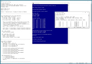 [Click on image for larger view.] Figure 1: Regression Using PyTorch Demo Run
After the training data is loaded into memory, the demo creates an 8-(10-10)-1 neural network. This means there are eight input nodes, two hidden neural layers with 10 nodes each and one output node.
The demo prepares to train the network by setting a batch size of 10, Adam (adaptive momentum) optimization with a learning rate of 0.01 and maximum training epochs of 1,000 passes through the training data. The meaning of these values and how they are determined will be explained shortly.
The demo program monitors training by computing and displaying loss values. The loss values slowly decrease which indicates that training is probably succeeding. The magnitude of the loss values isn't directly interpretable; the important thing is that the loss decreases.
After 1,000 training epochs, the demo program computes the accuracy of the trained model on the training data as 91 percent (182 out of 200 correct). The model accuracy on the test data is 85 percent (34 out of 40 correct). For regression problem accuracy, you must specify how close a prediction must be to the true value in order to be counted as a correct prediction. For the demo, a predicted income that's within 10 percent of the true value is counted as a correct prediction.
After evaluating the trained network, the demo predicts the income for a person who is male, 34 years old, from Oklahoma, who is a political moderate. The prediction is $45,392.60.
The demo concludes by saving the trained model to file so that it can be used later without having to retrain the network from scratch. There are two main ways to save a PyTorch model. The demo uses the save-state approach.
This article assumes you have a basic familiarity with Python and intermediate or better experience with a C-family language but does not assume you know much about PyTorch or neural networks. The complete demo program source code and data can be found at here. The first article in this two-part series describes data preparation and the neural network design.
Overall Program Structure
The overall structure of the demo program is presented in Listing 1. The demo program is named people_income.py. The program imports the NumPy (numerical Python) library and assigns it an alias of np. The program imports PyTorch and assigns it an alias of T. Most PyTorch programs do not use the T alias but my work colleagues and I often do so to save space. The demo program indents using two spaces rather than the more common four spaces, again to save space.
Listing 1: Overall Program Structure
# people_income.py
# predict income from sex, age, city, politics
# PyTorch 1.12.1-CPU Anaconda3-2020.02  Python 3.7.6
# Windows 10/11

import numpy as np
import torch as T
device = T.device('cpu')

class PeopleDataset(T.utils.data.Dataset): . . .

class Net(T.nn.Module): . . .

def accuracy(model, ds, pct_close): . . .
def accuracy_x(model, ds, pct_close): . . .
def train(model, ds, bs, lr, me, le): . . .

def main():
  # 0. get started
  print("Begin People predict income ")
  T.manual_seed(0)
  np.random.seed(0)

  # 1. create Dataset objects
  # 2. create network
  # 3. train model
  # 4. evaluate model accuracy
  # 5. make a prediction
  # 6. save model (state_dict approach)
  print("End People income demo ")

if __name__ == "__main__":
  main()
The demo places the control logic in a program-defined main() function. The training code is placed in a program-defined train() function. There are two program-defined functions to compute model accuracy. The accuracy() function works item-by-item and is useful for diagnosing incorrect predictions. The accuracy_x() function evaluates all data items at once and is faster than the accuracy() function.
The demo program begins by setting the seed values for the NumPy random number generator and the PyTorch generator. Setting seed values is helpful so that demo runs are mostly reproducible. However, when working with complex neural networks such as Transformer networks, exact reproducibility cannot always be guaranteed because of separate threads of execution.
Preparing to Train the Network
Training a neural network is the process of finding values for the weights and biases so that the network produces output that matches the training data. Most of the demo program code is associated with training the network. The terms network and model are often used interchangeably. In some development environments, network is used to refer to a neural network before it has been trained, and model is used to refer to a network after it has been trained.
The normalized and encoded training data looks like:
 1   0.24   1  0  0   0.2950   0  0  1
-1   0.39   0  0  1   0.5120   0  1  0
 1   0.63   0  1  0   0.7580   1  0  0
-1   0.36   1  0  0   0.4450   0  1  0
. . .
The fields are gender (-1 = male, +1 = female), age (divided by 100), state (Michigan = 100, Nebraska = 010, Oklahoma = 001), income (divided by 100,000) and political leaning (conservative = 100, moderate = 010, liberal = 001).
In the main() function, the training and test data are loaded into memory as Dataset objects, and then the training Dataset is passed to a DataLoader object:
  # 1. create Dataset and DataLoader objects
  print("Creating People train and test Datasets ")
  train_file = ".\\Data\\people_train.txt"
  test_file = ".\\Data\\people_test.txt"
  train_ds = PeopleDataset(train_file)  # 200 rows
  test_ds = PeopleDataset(test_file)    # 40 rows
  bat_size = 10
  train_ldr = T.utils.data.DataLoader(train_ds,
    batch_size=bat_size, shuffle=True)
Unlike Dataset objects that must be defined for each specific binary classification problem, DataLoader objects are ready to use as-is. The batch size of 10 is a hyperparameter. The special case when batch size is set to 1 is sometimes called online training.
Although not necessary, it's generally a good idea to set a batch size that evenly divides the total number of training items so that all batches of training data have the same size. In the demo, with a batch size of 10 and 200 training items, each batch will have 20 items. When the batch size doesn't evenly divide the number of training items, the last batch will be smaller than all the others. The DataLoader class has an optional drop_last parameter with a default value of False. If set to True, the DataLoader will ignore last batches that are smaller.
It's very important to explicitly set the shuffle parameter to True. The default value is False. When shuffle is set to True, the training data will be served up in a random order, which is what you want during training. If shuffle is set to False, the training data is served up sequentially. This almost always results in failed training because the updates to the network weights and biases oscillate, and no progress is made.
Creating the Network
The demo program creates the neural network like so:
  # 2. create neural network
  print("Creating 8-(10-10)-1 binary NN classifier ")
  net = Net().to(device)
  net.train()
The neural network is instantiated using normal Python syntax but with .to(device) appended to explicitly place storage in either "cpu" or "cuda" memory. Recall that device is a global-scope value set to "cpu" in the demo.
The network is set into training mode with the somewhat misleading statement net.train(). PyTorch neural networks can be in one of two modes, train() or eval(). The network should be in train() mode during training and eval() mode at all other times.
The train() vs. eval() mode is often confusing for people who are new to PyTorch in part because in many situations it doesn't matter what mode the network is in. Briefly, if a neural network uses dropout or batch normalization, then you get different results when computing output values depending on whether the network is in train() or eval() mode. But if a network doesn't use dropout or batch normalization, you get the same results for train() and eval() mode.
Because the demo network doesn't use dropout or batch normalization, it's not necessary to switch between train() and eval() mode. However, in my opinion it's good practice to always explicitly set a network to train() mode during training and eval() mode at all other times. By default, a network is in train() mode.
The train() method operates by reference and so the statement net.train() modifies the net object. If you are a fan of functional programming, you can write net = net.train() instead.
Training the Network
The train() function is presented in Listing 2. Training a neural network involves two nested loops. The outer loop iterates a fixed number of epochs (with a possible short-circuit exit). An epoch is one complete pass through the training data. The inner loop iterates through all batches of training data items.
Listing 2: Training the Network
def train(model, ds, bs, lr, me, le):
  # dataset, bat_size, lrn_rate, max_epochs, log interval
  train_ldr = T.utils.data.DataLoader(ds, batch_size=bs,
    shuffle=True)
  loss_func = T.nn.MSELoss()
  optimizer = T.optim.Adam(model.parameters(), lr=lr)

  for epoch in range(0, me):
    epoch_loss = 0.0  # for one full epoch
    for (b_idx, batch) in enumerate(train_ldr):
      X = batch[0]  # predictors
      y = batch[1]  # target income
      optimizer.zero_grad()
      oupt = model(X)
      loss_val = loss_func(oupt, y)  # a tensor
      epoch_loss += loss_val.item()  # accumulate
      loss_val.backward()  # compute gradients
      optimizer.step()     # update weights

    if epoch % le == 0:
      print("epoch = %4d  |  loss = %0.4f" % \
        (epoch, epoch_loss))
The train() function hard-codes the loss function (mean squared error) and optimizer (Adam). An alternative design is to pass these two objects as arguments to the train() function.
The enumerate() function returns the current batch index (0 through 19) and a batch of input values (sex, age, state, politics) with associated correct target income values. Using enumerate() is optional and you can skip getting the batch index by writing "for batch in train_ldr" instead.
The MSELoss() loss function returns a PyTorch tensor that holds a single numeric value. That value is extracted using the item() method so it can be accumulated as an ordinary non-tensor numeric value. In early versions of PyTorch, using the item() method was required but newer versions of PyTorch perform an implicit type-cast so the call to item() is not necessary. In my opinion, explicitly using the item() method is better coding style.
The backward() method computes gradients. Each weight and bias has an associated gradient. Gradients are numeric values that indicate how an associated weight or bias should be adjusted so that the error/loss between computed outputs and target outputs is reduced. It's important to remember to call the zero_grad() method before calling the backward() method. The step() method uses the newly-computed gradients to update the network weights and biases.
Most neural binary regression models can be trained in a relatively short time. In situations where training takes several hours or longer, you should periodically save the values of the weights and biases so that if your machine fails (loss of power, dropped network connection and so on) you can reload the saved checkpoint and avoid having to restart from scratch.
Saving a training checkpoint is outside the scope of this article. For an example and explanation of saving training checkpoints, see my blog post.
The statements that train the regression model are:
  # 3. train model
  print("bat_size = 10 ")
  print("loss = MSELoss() ")
  print("optimizer = Adam ")
  print("lrn_rate = 0.01 ")

  print("Starting training")
  net.train()  # set mode
  train(net, train_ds, bs=10, lr=0.01, me=1000, le=100)
  print("Done ")
The maximum number of epochs to train (me) is a hyperparameter that must be determined by trial and error. The log interval (le) specifies how often to display progress messages.
The demo uses Adam (adaptive momentum) optimization with a fixed learning rate of 0.01 that controls how much weights and biases change on each update. PyTorch supports 13 different optimization algorithms. The two most common are SGD and Adam (adaptive moment estimation). SGD often works reasonably well for simple networks. Adam often, but not always, works better than SGD for deep neural networks.
PyTorch beginners sometimes fall into a trap of trying to learn everything about every optimization algorithm. Most of my experienced colleagues use just two or three algorithms and adjust the learning rate. My recommendation is to use SGD and Adam and try other algorithms only when those two fail.
It's important to monitor training progress, because training failure is the norm rather than the exception. There are several ways to monitor training progress. The demo program uses the simplest approach, which is to accumulate the total loss for one epoch and then display that accumulated loss value every so often (every 100 epochs in the demo).
Computing Model Accuracy
You must implement a program-defined accuracy() function for regression problems. Because the output and target values of a regression model are numeric values, you must specify how close a predicted value must be to its target value in order for the prediction to be counted as correct. For example, if a target income is 0.6000 ($60,000.00) and you specify a 10 percent closeness interval, then predictions between 0.5400 and 0.6600 would be scored as correct.
The code in Listing 3 shows a simple accuracy function that works item-by-item. This approach is slow but allows you to insert print statements to diagnose incorrect predictions.
Listing 3: A Simple Accuracy Function
def accuracy(model, ds, pct_close):
  n_correct = 0; n_wrong = 0
  for i in range(len(ds)):
    X = ds[i][0]   # 2-d inputs
    Y = ds[i][1]   # 2-d target
    with T.no_grad():
      oupt = model(X)  # computed income

    if T.abs(oupt - Y) < T.abs(pct_close * Y):
      n_correct += 1
    else:
      n_wrong += 1
  acc = (n_correct * 1.0) / (n_correct + n_wrong)
  return acc
The code in Listing 4 shows an accuracy function that works with all inputs and outputs at once, and so is faster than the item-by-item approach. This is useful when you just want an accuracy result quickly.
Listing 4: A Fast Accuracy Function
def accuracy_x(model, ds, pct_close):
  X = ds.x_data  # all inputs
  Y = ds.y_data  # all targets
  n_items = len(X)
  with T.no_grad():
    pred = model(X)  # all predicted incomes

  n_correct = T.sum((T.abs(pred - Y) < T.abs(pct_close * Y)))
  result = (n_correct.item() / n_items)  # scalar
  return result
The demo program calls the two accuracy functions like so:
  # 4. evaluate model accuracy
  print("Computing model accuracy (within 0.10 of true) ")
  net.eval()
  acc_train = accuracy(net, train_ds, 0.10)  # item-by-item
  print("Accuracy on train data = %0.4f" % acc_train)
  acc_test = accuracy_x(net, test_ds, 0.10)  # all-at-once/
  print("Accuracy on test data = %0.4f" % acc_test)
Notice that the calling code places the network in eval() mode before calling the accuracy functions. As explained earlier, this is not necessary because the network doesn't use dropout or batch normalization.
Using the Model
After the network regression model has been trained, the demo uses the model to make an income prediction for a new, previously unseen person:
  # 5. make a prediction
  print("Predicting income for M 34 Oklahoma moderate: ")
  x = np.array([[-1, 0.34, 0,0,1, 0,1,0]],
    dtype=np.float32)
  x = T.tensor(x, dtype=T.float32).to(device)
  with T.no_grad():
    pred_inc = net(x)
  pred_inc = pred_inc.item()  # scalar
  print("$%0.2f" % (pred_inc * 100_000))  # un-normalized
The input is a person who is male, 34 years old, lives in Oklahoma and is a political moderate. Because the network was trained on normalized and encoded data, the input must be normalized and encoded in the same way.
Notice the double set of square brackets. A PyTorch network expects input to be in the form of a batch. The extra set of brackets creates a data item with a batch size of 1. Details like this can take a lot of time to debug.
Because the neural network has no activation on the output node, the predicted income is in normalized form. The demo un-normalizes the predicted income by multiplying by $100,000.
Saving the Trained Model
The demo program concludes by saving the trained model using these statements:
  # 6. save model (state_dict approach)
  print("Saving trained model state")
  fn = ".\\Models\\people_income_model.pt"
  T.save(net.state_dict(), fn)
The code assumes there is a directory named Models. There are two main ways to save a PyTorch model. You can save just the weights and biases that define the network, or you can save the entire network definition including weights and biases. The demo uses the first approach.
The model weights and biases, along with some other information, is saved in the state_dict() Dictionary object. The torch.save() method accepts the Dictionary and a file name that indicates where to save. You can use any file name extension you wish but .pt and .pth are two common choices.
To use the saved model from a different program, that program would have to contain the network class definition. Then the weights and biases could be loaded like so:
model = Net()  # requires class definition
model.eval()
fn = ".\\Models\\people_income_model.pt"
model.load_state_dict(T.load(fn))
# use model to make prediction(s)
When saving or loading a trained model, the model should be in eval() mode rather than train() mode. An alternative approach for saving a PyTorch model is to use ONNX (Open Neural Network Exchange). This allows cross platform usage.
Wrapping Up
The term regression has multiple meanings in machine learning. This article has described general regression where the goal is to predict a single numeric value such a person's income.
Simple linear regression is a classical statistics technique that predicts a single numeric value from just one numeric predictor variable, for example, predicting income from age. Multiple linear regression is a classical statistics technique that predicts a single numeric value from two or more numeric predictor variables, for example, predicting income from age and height.
Logistic regression, in spite of its name, is actually a binary classification technique, for example, predicting sex (male = 0, female = 1) from age and income. The output of a logistic regression model is a single numeric value between 0 and 1 (hence the term regression), but the output value is a pseudo-probability where values less than 0.5 indicate class 0 and values greater than 0.5 indicate class 1 (and so it's a classification technique).