The Data Science Lab
Regression Using PyTorch, Part 1: New Best Practices
Machine learning with deep neural techniques has advanced quickly, so Dr. James McCaffrey of Microsoft Research updates regression techniques and best practices guidance based on experience over the past two years.
A regression problem is one where the goal is to predict a single numeric value. For example, you might want to predict the annual income of a person based on their sex, age, state where they live and political leaning (conservative, moderate, liberal).
A previous article series in Visual Studio Magazine have explained regression using PyTorch. But machine learning with deep neural techniques has advanced quickly. This article updates regression techniques and best practices based on experience over the past two years.
A good way to see where this article is headed is to take a look at the screenshot of a demo program in Figure 1. The demo begins by loading a 200-item file of training data and a 40-item set of test data. Each tab-delimited line represents a person. The fields are sex (male = -1, female = +1), age, state of residence, annual income and politics type. The goal is to predict income from sex, age, state, and political leaning.
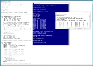 [Click on image for larger view.] Figure 1: Regression Using PyTorch Demo Run
After the training data is loaded into memory, the demo creates an 8-(10-10)-1 neural network. This means there are eight input nodes, two hidden neural layers with 10 nodes each, and one output node.
The demo prepares to train the network by setting a batch size of 10, Adam (adaptive momentum) optimization with a learning rate of 0.01, and maximum training epochs of 1,000 passes through the training data. The meaning of these values and how they are determined will be explained shortly.
The demo program monitors training by computing and displaying loss values. The loss values slowly decrease which indicates that training is probably succeeding. The magnitude of the loss values isn't directly interpretable; the important thing is that the loss decreases.
After 1,000 training epochs, the demo program computes the accuracy of the trained model on the training data as 91 percent (182 out of 200 correct). The model accuracy on the test data is 85 percent (34 out of 40 correct). For regression problem accuracy, you must specify how close a prediction must be to the true value in order to be counted as a correct prediction. For the demo, a predicted income that's within 10 percent of the true value is counted as a correct prediction.
After evaluating the trained network, the demo predicts the income for a person who is male, 34 years old, from Oklahoma, who is a political moderate. The prediction is $45,392.60.
The demo concludes by saving the trained model to file so that it can be used later without having to retrain the network from scratch. There are two main ways to save a PyTorch model. The demo uses the save-state approach.
This article assumes you have a basic familiarity with Python and intermediate or better experience with a C-family language but does not assume you know much about PyTorch or neural networks. The complete demo program source code and data can be found here.
Installing PyTorch
The demo program was developed on a Windows 10/11 machine using the Anaconda 2020.02 64-bit distribution (which contains Python 3.7.6) and PyTorch version 1.12.1 for CPU. Installing PyTorch is like swimming -- easy once you know how but difficult if you haven't done it before.
I work at a large tech company and one of my job responsibilities is to deliver training classes to software engineers and data scientists. By far the biggest hurdle for people who are new to PyTorch is installation.
There are dozens of different ways to install PyTorch on Windows. The configuration I strongly recommend for beginners is to use the Anaconda distribution of Python and install PyTorch using the pip package manager. The Anaconda distribution of Python contains a base Python engine plus over 500 add-in packages that have been tested to be compatible with one another.
After you have a Python distribution installed, you can install PyTorch in several different ways. I recommend using the pip utility, which is installed as part of Anaconda. Briefly, you download a .whl ("wheel") file to your local machine, open a command shell and issue the command "pip install (whl-file-name)."
You can find detailed step-by-step instructions for installing Anaconda Python for Windows 10/11 here. You can find detailed instructions for downloading and installing PyTorch 1.12.1 for Python 3.7.6 on a Windows CPU machine here.
Preparing the Data
The raw demo data looks like:
F   24   michigan   29500.00   liberal
M   39   oklahoma   51200.00   moderate
F   63   nebraska   75800.00   conservative
M   36   michigan   44500.00   moderate
. . .
There are 240 lines of data. Each line represents a person. The five fields are sex (M, F), age, state of residence (Michigan, Nebraska, Oklahoma), annual income and politics type (conservative, moderate, liberal). The data is artificial. The raw data was split into a 200-item set for training and a 40-item set for testing.
The raw data must be encoded and normalized. The result is:
 1   0.24   1  0  0   0.2950   0  0  1
-1   0.39   0  0  1   0.5120   0  1  0
 1   0.63   0  1  0   0.7580   1  0  0
-1   0.36   1  0  0   0.4450   0  1  0
. . .
The variable to predict is income, which is a numeric value rather than a categorical value such as sex or political leaning. Notice that the income values are normalized by dividing the raw values by $100,000. In theory this isn't necessary, but normalizing regression target values to a -1.0 to +1.0 range or -10.0 to +10.0 range usually helps.
Because neural networks only understand numbers, the sex, state and political leaning predictor values (often called features in neural network terminology) must be encoded. The sex values are minus-one-plus-one encoded rather than 0-1 encoding. In theory both encoding schemes work for binary predictor variables but in practice minus-one-plus-one encoding often produces a better model. For an explanation, go here.
The demo normalizes the age values by dividing each raw value by 100. The technique of normalizing numeric predictors by dividing them by a constant does not have a standard name. Two other normalization techniques are called min-max normalization and z-score normalization. I recommend using the divide-by-constant technique whenever possible. There is convincing (but currently unpublished) research that indicates divide-by-constant normalization usually gives better results than min-max normalization or z-score normalization. The topic is quite complex. For details, go here.
The state of residence values are one-hot encoded as Michigan = (1 0 0), Nebraska = (0 1 0) and Oklahoma = (0 0 1). The order of the encoding is arbitrary. If the state variable had four possible values, then the encodings would be (1 0 0 0), (0 1 0 0) and so on. The political leaning values are one-hot encoded as conservative = (1 0 0), moderate = (0 1 0) and liberal = (0 0 1).
The demo preprocesses the raw data by normalizing numeric values and encoding categorical values. It is possible to normalize and encode training and test data on the fly, but preprocessing is usually a simpler approach.
Overall Program Structure
The overall structure of the demo program is presented in Listing 1. The demo program is named people_income.py. The program imports the NumPy (numerical Python) library and assigns it an alias of np. The program imports PyTorch and assigns it an alias of T. Most PyTorch programs do not use the T alias but my work colleagues and I often do so to save space. The demo program indents using two spaces rather than the more common four spaces, again to save space.
Listing 1: Overall Program Structure
# people_income.py
# predict income from sex, age, city, politics
# PyTorch 1.12.1-CPU Anaconda3-2020.02  Python 3.7.6
# Windows 10/11

import numpy as np
import torch as T
device = T.device('cpu')

class PeopleDataset(T.utils.data.Dataset): . . .

class Net(T.nn.Module): . . .

def accuracy(model, ds, pct_close): . . .
def accuracy_x(model, ds, pct_close): . . .
def train(model, ds, bs, lr, me, le): . . .

def main():
  # 0. get started
  print("Begin People predict income ")
  T.manual_seed(0)
  np.random.seed(0)

  # 1. create Dataset objects
  # 2. create network
  # 3. train model
  # 4. evaluate model accuracy
  # 5. make a prediction
  # 6. save model (state_dict approach)

  print("End People income demo ")

if __name__ == "__main__":
  main()
The global device is set to "cpu." If you are working with a machine that has a GPU processor, the device string is "cuda." Most of my colleagues and I develop neural networks on a local CPU machine, then if necessary (huge amount of training data or huge neural network), push the program to a GPU machine and train it there.
The demo has a program-defined PeopleDataset class that stores training and test data. Data in a Dataset object can be served up in batches for training by using the built-in DataLoader object. It is possible to use training and test data directly instead of using a Dataset, but such problem scenarios are rare and I recommend using a Dataset for most problems.
The regression neural network is implemented in a program-defined Net class. The Net class inherits from the built-in torch.nn.Module class, which supplies most of the neural network functionality. Instead of using a class to define a PyTorch neural network, it is possible to create a neural network directly using the torch.nn.Sequential class. Using Sequential is simpler but less flexible than using a program-defined class. The fact that there are two completely different ways to define a PyTorch neural network can be confusing for beginners.
In a neural network regression problem, you must implement a program-defined function to compute the accuracy of the trained model. The demo program defines an accuracy() function that works line-by-line, and an accuracy_x() function that works on all data at once.
The demo implements a program-defined train() function. In most cases, I just place all training code directly inside the main() function, but using a train() function is preferred by many of my colleagues.
All of the demo program control logic is contained in a program-defined main() function. The demo program begins by setting the seed values for the NumPy random number generator and the PyTorch generator. Setting seed values is helpful so that demo runs are mostly reproducible. However, when working with complex neural networks such as Transformer networks, exact reproducibility cannot always be guaranteed because of separate threads of execution.
The Dataset Definition
The demo Dataset definition is presented in Listing 2. A Dataset inherits from the torch.utils.data.Dataset class and you must implement three methods: __init__(), __len__(), and __getitem__(). The __init__() method loads the data from file into memory as PyTorch tensors. The __len__() method tells the DataLoader object that uses the Dataset how many items there so that the DataLoader knows when all items have been processed during training. The __getitem__() method returns a single data item, rather than a batch of items as you might have expected.
Listing 2: Dataset Definition
class PeopleDataset(T.utils.data.Dataset):
  def __init__(self, src_file):
    # like: -1  0.27  0 1 0   0.7610   0 0 1
    tmp_x = np.loadtxt(src_file, usecols=[0,1,2,3,4,6,7,8],
      delimiter="\t", comments="#", dtype=np.float32)
    tmp_y = np.loadtxt(src_file, usecols=5, delimiter="\t",
      comments="#", dtype=np.float32)
    tmp_y = tmp_y.reshape(-1,1)  # 2D required

    self.x_data = T.tensor(tmp_x, dtype=T.float32).to(device)
    self.y_data = T.tensor(tmp_y, dtype=T.float32).to(device)

  def __len__(self):
    return len(self.x_data)

  def __getitem__(self, idx):
    preds = self.x_data[idx]
    incom = self.y_data[idx]
    return (preds, incom)  # as a tuple
Defining a PyTorch Dataset is not trivial. You must define a custom Dataset for each problem/data scenario. The __init__() method accepts a src_file parameter that tells the Dataset where the file of training data is located. The predictor values and the target income values are read into tmp_x and tmp_y as NumPy matrices in two separate passes. Then the NumPy matrices are converted to PyTorch tensors.
An alternative design is to read predictor and target values in one pass, then extract. Code would look like:
all_xy = np.loadtxt(src_file, usecols=[0,1,2,3,4,5,6,7,8],
  delimiter="\t", comments="#", dtype=np.float32)
tmp_x = all_xy[:,[0,1,2,3,4,6,7,8]]
tmp_y = all_xy[:,5].reshape(-1,1)  # 2D required
The demo reads data using the NumPy loadtxt() function. Commonly used alternatives include the NumPy genfromtxt() function and the Pandas read_csv() function.
The call to loadtxt() specifies argument comments="#" to indicate that lines beginning with "#" are comments and should be ignored. The "#" character is the default for comments and so the argument could have been omitted.
Notice that both the predictors and the target incomes are stored as float32 values. This is the default floating point type, unlike float64 as you might expect if you're new to PyTorch.
The target income values are stored in a two-dimensional matrix rather than a one-dimensional vector. This is required by PyTorch. Dealing with PyTorch vector and matrix shapes can be extremely time-consuming during development.
The self.x_data and self.y_data are stored in memory using the .to(device) method which in this case is "cpu." Because the default device type for a newly created PyTorch Tensor object is None, it's good practice to explicitly use .to(device) whenever a new Tensor is instantiated.
The __len__() function returns the number of rows in the self.x_data Tensor matrix. You could also use len(self.y_data) because the self.y_data vector has the same number of values.
The __getitem__() method accepts an index parameter, idx. The predictor values for item [idx] are pulled from self.x_data using normal array indexing. The target income values are also pulled using normal indexing syntax. The return value is a Python Tuple object where a set of predictors values is at tuple position [0] and the single associated target income is at tuple position [1].
An alternative approach is to return the predictors and label as a Python Dictionary object. That code would look like:
def __getitem__(self, idx):
  preds = self.x_data[idx]
  incom = self.y_data[idx]
  sample = { 'predictors' : preds, 'targets' : incom }
  return sample  # as Dictionary
The Dictionary approach allows you to access predictors and labels by name rather than by indexing. However, the Dictionary approach creates "magic strings" and so the Tuple approach is more common, at least among my colleagues.
The demo Dataset definition assumes that the predictor values and the class labels are in the same source file. In some situations, the predictors and label are defined in separate files. In such situations you must pass two file paths instead of just one to the __init__() method.
A Dataset must be able to store all data in memory. This usually isn't a problem. But for huge sets of data, you must create a streaming data loader. This is difficult. See "How To: Create a Streaming Data Loader for PyTorch" for an example.
Defining the Network
The neural network definition is presented in Listing 3. The network architecture is 8-(10-10)-1 with tanh() hidden node activation. The number of input nodes for a regression problem is determined by the training data. There is always one output node. The number of hidden layers and the number of nodes in each layer are hyperparameters that must be determined by trial and error.
The __init__() method sets up the layers and optionally specifies how to initialize the layer weights and biases. The demo uses explicit initialization, but it's more common to use default weight and bias initialization. Weight and bias initialization is a surprisingly complex topic, and the documentation on the topic is a weak point of PyTorch. The choice of initialization algorithm often has a big effect on the behavior of a neural network.
The advantage of using default weight and bias initialization is simplicity. The disadvantage is that the default initialization algorithm can, and has, changed several times. My recommendation is to use explicit weight and bias initialization for simple regression problems with just one or two hidden layers, but use default initialization for classifiers with three or more hidden layers.
Listing 3: Neural Network Class Definition
class Net(T.nn.Module):
  def __init__(self):
    super(Net, self).__init__()
    self.hid1 = T.nn.Linear(8, 10)  # 8-(10-10)-1
    self.hid2 = T.nn.Linear(10, 10)
    self.oupt = T.nn.Linear(10, 1)

    T.nn.init.xavier_uniform_(self.hid1.weight)
    T.nn.init.zeros_(self.hid1.bias)
    T.nn.init.xavier_uniform_(self.hid2.weight)
    T.nn.init.zeros_(self.hid2.bias)
    T.nn.init.xavier_uniform_(self.oupt.weight)
    T.nn.init.zeros_(self.oupt.bias)

  def forward(self, x):
    z = T.tanh(self.hid1(x))
    z = T.tanh(self.hid2(z))
    z = self.oupt(z)  # regression: no activation
    return z
The demo network uses tanh() activation on the hidden nodes. In the early days of neural networks, sigmoid() hidden layer activation was common, but it's now rarely used. For deep neural networks, relu() activation is often used. There are essentially no good rules of thumb for deciding which hidden layer activation to use. It's a good idea to try both tanh() and relu() and see which seems to work better in combination with all your other hyperparameters.
A common source of confusion for people who are new to PyTorch is the output layer activation function. There is a strong coupling between output activation and the loss function used during training. The demo program uses no output layer activation, which means output values can range between minus infinity to plus infinity. Because all normalized target income values are between 0 and 1, it seems logical to apply sigmoid() activation on the output node. However, this just didn't work as well as no activation.
The network dimensions of 8, 10, 10 and 1 are hard-coded. It is possible to pass these values as parameters to the __init__() function, but the hard-coded approach is simpler and easier to understand, which trumps the minor loss of flexibility in my opinion.
Wrapping Up
The demo code presented in this article can be used as a guide to prepare training data and a template to define a neural network for most regression problems. Part 2 will explain how to train the network, compute the trained network's accuracy, save the network for use by other programs, and use the network to make predictions.