The Data Science Lab
Naive Bayes Classification Using the scikit Library
Dr. James McCaffrey of Microsoft Research shows how to predict a person's sex based on their job type, eye color and country of residence.
Naive Bayes classification is a classical machine learning technique to predict a discrete value. For example, you might want to predict the sex of a person (female or male) based on their job type, eye color and country of residence. In addition to binary classification, naive Bayes can also be used for multi-class classification, for example, predicting job type (actuary, barista, chemist, dentist) from eye color, country and sex.
Naive Bayes classification is especially well suited to problems where the predictor variables are all categorical (strings). And, compared to neural network classifiers, naive Bayes classifications can work well with small training datasets.
There are several tools and code libraries that you can use to perform naive Bayes classification. The scikit-learn library (also called scikit or sklearn) is based on the Python language and is one of the most popular machine learning libraries.
A good way to see where this article is headed is to take a look at the screenshot in Figure 1. The demo program begins by loading a synthetic 20-item set training data into memory. The goal is to predict the sex of a person (female = 0, male = 1) from job type, eye color and country. The demo echoes the predictor values and the target class labels. A naive Bayes classifier is created and then used to make predictions for the 20 data items.
The accuracy of the trained model is 80 percent (16 out of 20 correct). The demo displays a confusion matrix for the model predictions:
actual = 0  [11  1]
actual = 1  [ 3  5]
predicted:    0  1
The model correctly predicted 11 class 0 (female) data items and incorrectly predicted one class 0 item. The model correctly predicted five of the eight class 1 (male) data items.
The demo concludes by predicting the sex/class/label for a new, previously unseen data item of (dentist, hazel, Italy). The model displays the prediction in the form of a vector of pseudo-probabilities: [0.33, 0.67]. Because the larger pseudo-probability is at index [1], the prediction is class 1 = male.
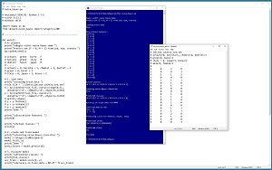 [Click on image for larger view.] Figure 1: Naive Bayes Classification Using scikit in Action
This article assumes you have intermediate or better skill with a C-family programming language such as Python or C#, but doesn't assume you know much about naive Bayes classification or the scikit library. The complete source code for the demo program is presented in this article. The source code is also available in the accompanying file download and is also available online.
Installing the scikit Library
There are several ways to install the scikit library. I recommend installing the Anaconda Python distribution. Anaconda contains a core Python engine plus more than 500 libraries that are (mostly) compatible with each other. I used Anaconda3-2020.02, which contains Python 3.7.6 and the scikit 0.22.1 version. The demo code runs on Windows 10 or 11.
Briefly, Anaconda is installed using a Windows self-extracting executable file. The setup process is mostly straightforward and takes about 15 minutes. You can consult step-by-step instructions.
There are more up-to-date versions of Anaconda/Python/scikit library available. But because the Python ecosystem has hundreds of libraries, if you install the most recent versions of these libraries, you run a greater risk of library incompatibilities -- a major headache when working with Python.
The Data
The 20-item raw source data is shown in Listing 1. Notice that all values are strings. If source data contains a predictor column where the values are numeric, then those values should be converted to strings by bucketing them. For example, if the raw source data had a person's age column with values like 24 and 37, then you could bucket the age values along the lines of "young" = ages 18 through 29, "middle" = ages 30 through 59 and "old" = ages 60 through 99.
Listing 1: The Raw Source Data
actuary   green   korea   F
barista   green   italy   M
dentist   hazel   japan   M
dentist   green   italy   F
chemist   hazel   japan   M
actuary   green   japan   F
actuary   hazel   japan   M
chemist   green   italy   F
chemist   green   italy   F
dentist   green   japan   F
barista   hazel   japan   M
dentist   green   japan   F
dentist   green   japan   F
chemist   green   italy   F
dentist   green   japan   M
dentist   hazel   japan   M
chemist   green   korea   F
barista   green   japan   F
actuary   hazel   italy   F
actuary   green   italy   M
When working with naive Bayes, the data should be integer-encoded as shown in Listing 2. Integer-encoding is sometimes called ordinal encoding or label encoding.
Listing 2: The Integer/Ordinal Encoded Data
# job_eye_country_sex.txt
# actuary=0, barista=1, chemist=2, dentist=3
# green=0, hazel=1
# italy = 0, japan=1, korea=2
# female=0, male=1
#
0   0   2   0
1   0   0   1
3   1   1   1
3   0   0   0
2   1   1   1
0   0   1   0
0   1   1   1
2   0   0   0
2   0   0   0
3   0   1   0
1   1   1   1
3   0   1   0
3   0   1   0
2   0   0   0
3   0   1   1
3   1   1   1
2   0   2   0
1   0   1   0
0   1   0   0
0   0   0   1
The "#" character indicates a comment line. The demo data is tab-separated and saved as job_eye_country_sex.txt, so if you copy-paste from this article you'll need to replace the spaces with tab characters or modify the demo code that loads the data into memory. Notice that the values in each column are encoded based on alphabetical order. This is standard procedure when working with naive Bayes but is not required.
Encoding the data from strings to integers is simple but time-consuming. The data can be encoded manually, for example by dropping the string data into an Excel spreadsheet and then applying find-replace operations.
It is also possible to programmatically encode string data using the scikit OrdinalEncoder class or by using a program-defined function. These two approaches will be explained shortly.
Understanding How Naive Bayes Classification Works
Understanding how naive Bayes classification works is best explained by example. Suppose, as in the demo program, the goal is to predict the sex of a person who is a dentist, has hazel colored eyes and who lives in Italy.
If you look just at the dentists in the job column, three of the seven dentists are male, and four of the seven are female. So you'd (weakly) guess the person is female. Next, if you look just at the hazel values in eye color column, five of six people are male and just one of six are female. So based just on eye color you'd strongly guess male. And then, if you look just at the Italy values in the country column, two of seven people are male and five of seven are female. So you'd guess the person is female.
If the frequencies are loosely interpreted as pseudo-probabilities, then:
Job: P(female) = 0.57  P(male) = 0.43
Eye: P(female) = 0.17  P(male) = 0.83
Cty: P(female) = 0.71  P(male) = 0.29
Therefore the job type and country predictors suggest the (dentist, hazel, Italy) person is female, but the eye color predictor strongly suggests the person is male. A simple way to produce a single prediction is to use a majority-rule vote. However, this approach isn't very good because different predictor distributions should be weighted differently. For example, suppose there is a height column with values "short," "medium" and "tall." If most of the data items are "short" or "medium," then a data item with height value of "tall" contains more information and should receive more weight.
The naive Bayes technique combines the frequencies in each predictor column in a way that takes relative frequencies into account. The technique is called "naive" (meaning unsophisticated) because each predictor column is analyzed independently, not taking into account interactions between columns. The name "Bayes" refers to Thomas Bayes (1701-1761), a founder of probability theory.
The Demo Program
The complete demo program is presented in Listing 3. I am a proud user of Notepad as my preferred code editor, but most of my colleagues use a more sophisticated programming environment. I indent my Python program using two spaces rather than the more common four spaces.
The program imports the NumPy library, which contains numeric array functionality. The CategoricalNB module has the key code for performing naive Bayes classification. Notice the name of the root scikit module is sklearn rather than scikit.
Listing 3: Complete Naive Bayes Demo Program
# naive_bayes.py

# Anaconda3-2020.02  Python 3.7.6
# scikit 0.22.1
# Windows 10/11

import numpy as np
from sklearn.naive_bayes import CategoricalNB

# ---------------------------------------------------------

def main():
  # 0. prepare
  print("\nBegin scikit naive Bayes demo ")
  print("Predict sex (F = 0, M = 1) from job, eye, country ")
  np.random.seed(1)

  # actuary   green   korea   F
  # barista   green   italy   M
  # dentist   hazel   japan   M
  # . . .
  # actuary = 0, barista = 1, chemist = 2, dentist = 3
  # green = 0, hazel = 1
  # italy = 0, japan = 1, korea = 2

  # 1. load data
  print("\nLoading train data ")
  train_file = ".\\Data\\job_eye_country_sex.txt"
  X = np.loadtxt(train_file, usecols=range(0,3),
    delimiter="\t", comments="#", dtype=np.int64)
  y = np.loadtxt(train_file, usecols=3,
    delimiter="\t", comments="#", dtype=np.int64)
  print("Done ")

  print("\nDiscretized features: ")
  print(X)

  print("\nActual classes: ")
  print(y)

  # 2. create and train model
  print("\nCreating naive Bayes classifier ")
  model = CategoricalNB(alpha=1)
  model.fit(X, y)
  print("Done ")
  pred_classes = model.predict(X)

  # 3. evaluate model
  print("\nPredicted classes: ")
  print(pred_classes)
  acc_train = model.score(X, y)
  print("\nAccuracy on train data = %0.4f " % acc_train)

  # 3b. confusion matrix
  from sklearn.metrics import confusion_matrix
  y_predicteds = model.predict(X)
  cm = confusion_matrix(y, y_predicteds)  # actual, pred
  print("\nConfusion matrix raw: ")
  print(cm)

  # 4. use model
  # dentist, hazel, Italy = [3,1,0]
  print("\nPredicting class for dentist, hazel, Italy ")
  probs = model.predict_proba([[3,1,0]])
  print("\nPrediction probs: ")
  print(probs)

  predicted = model.predict([[3,1,0]])
  print("\nPredicted class: ")
  print(predicted)

  # 5. TODO: save model using pickle

  print("\nEnd demo ")

if __name__ == "__main__":
  main()
The demo begins by setting the NumPy random seed:
def main():
  # 0. prepare
  print("Begin scikit naive Bayes demo ")
  print("Predict sex (F=0, M=1) from job, eye, country ")
  np.random.seed(1)
. . .
Technically, setting the random seed value isn't necessary, but doing so allows you to get reproducible results in many situations.
Loading the Training and Test Data
The demo program loads the training data into memory using these statements:
  # 1. load data
  print("Loading train data ")
  train_file = ".\\Data\\job_eye_country_sex.txt"
  X = np.loadtxt(train_file, usecols=range(0,3),
    delimiter="\t", comments="#", dtype=np.int64)
  y = np.loadtxt(train_file, usecols=3,
    delimiter="\t", comments="#", dtype=np.int64)
  print("Done ")
This code assumes the data files are stored in a directory named Data. There are many ways to load data into memory. I prefer using the NumPy library loadtxt() function, but common alternatives are the NumPy genfromtxt() function and the Pandas library read_csv() function.
The demo reads the predictors and the target class labels using two calls to the loadtxt() function. Because the demo data has predictors and labels in the same file, an alternative is to read both using one call to loadtxt() and then extract like so:
XY = np.loadtxt(train_file, usecols=range(0,4),
  delimiter="\t", comments="#", dtype=np.int64)
X = XY[:,0:3]
y = XY[:,3]
The colon syntax means "all rows." The demo program does not have any test data, but test data would be read into memory in the same way as the training data.
The demo program prints the 20 encoded predictor items and the 20 target gender values:
  print("Discretized features: ")
  print(X)
  print("Actual classes: ")
  print(y)
In a non-demo scenario with a lot of training data, you might want to display just part of the data.
Programmatically Converting Raw String Data to Integers
The demo program assumes the existence of manually encoded integer/ordinal data. One way to programmatically encode raw string data for use by a scikit naive Bayes classifier is to use the OrdinalEncoder class. Suppose the raw data is stored in a text file named job_eye_country_sex_raw.txt and looks like:
actuary   green   korea   F
barista   green   italy   M
dentist   hazel   japan   M
. . .
To programmatically encode the strings to integer values you could write code like:
from sklearn.preprocessing import OrdinalEncoder
train_file = ".\\Data\\job_eye_country_sex_raw.txt"
raw = np.genfromtxt(train_file, usecols=range(0,4),
  delimiter="\t", dtype=str)
enc.fit(raw)  # scan data
encoded = enc.transform(raw)  # encode the data
X = encoded[:,0:3]
y = encoded[:,3]
Notice the NumPy genfromtxt() function is used rather than the loadtxt() function because loadtxt() does not support reading string ("str") data.
The OrdinalEncoder class is simple to use, but it isn't easy to customize how strings are encoded. It's not too difficult to write a program-defined function to encode string data to integer data. See my guidance.
Creating and Training the Model
Creating and training the naive Bayes classification model is relatively simple:
  # 2. create and train model
  print("Creating naive Bayes classifier ")
  model = CategoricalNB(alpha=1)
  model.fit(X, y)
  print("Done ")
  pred_classes = model.predict(X)
Unlike many scikit models, the CategoricalNB class has relatively few -- just four -- parameters (Note: newer versions of scikit have an additional min_categories parameter, which isn't very useful):
CategoricalNB(*, alpha=1.0, force_alpha='warn', fit_prior=True, class_prior=None)
When working with scikit, you'll spend most of your time reading the documentation and trying to figure out what each model parameter does. The alpha parameter is a bit tricky to explain. Because naive Bayes computes many frequencies based on counts of data, it's very possible for the denominator of a frequency to be zero, which will throw a division-by-zero error. Behind the scenes, the alpha value is added to all counts to ensure that there will never be that error. This technique is called Laplacian smoothing. Notice that the default value of alpha is 1.0 so the demo code could have omitted the explicit argument.
The default value of the fit_prior parameter is True. This means that by default the initial relative frequencies of the predictor variables are computed based on the data. For example, the demo data country column has seven Italy values, 11 Japan values and two Korea values, so the initial relative frequency of Italy is 7 / 20 = 0.35. If you specify fit_prior=False, then all initial values in a column are assumed to be equal. In this example, the initial frequencies of Italy, Japan and Korea would all be set to 0.33.
The default value of the class_prior is None. This means that by default the initial relative frequencies of the variable to predict are based on the data. So, because the demo data has 12 female and eight male items, the initial relative frequency of female is 12 / 20 = 0.60, and the initial relative frequency of male is 8 / 20 = 0.40. If you specify initial values for the class_prior parameter, those values will be used instead. For example, class_prior = [0.50, 0.50] will set the initial relative frequencies of both female and male to 0.50.
After everything has been prepared, the model is trained using the fit() method. It's almost too easy. After the model has been trained, it's used to predict the class labels of all 20 data items.
Evaluating the Trained Model
The demo computes the accuracy of the trained model like so:
  # 3. evaluate model
  print("Predicted classes: ")
  print(pred_classes)
  acc_train = model.score(X, y)
  print("Accuracy on train data = %0.4f " % acc_train)
The score() function computes a simple accuracy, which is just the number of correct predictions divided by the total number of predictions. However, for binary classification problems you usually want additional evaluation metrics due to the possibility of unbalanced data. Suppose the 20-item training data had 18 males and just two females. A model that predicts male for any set of inputs would always achieve 18 / 20 = 90 percent accuracy.
Three common evaluation metrics that provide additional information are precision, recall and F1 score. The scikit library has several ways to compute these. A simple technique is:
from sklearn.metrics import classification_report
report = classification_report(y, pred_classes)  # actual, predicted
print(report)
In general you should examine precision and recall and only be concerned when either is very low. The F1 score metric is just the harmonic mean of precision and recall.
The demo prints a confusion matrix:
  # 3b. confusion matrix
  from sklearn.metrics import confusion_matrix
  y_predicteds = model.predict(X)
  cm = confusion_matrix(y, y_predicteds)  # actual, predicted
  print("Confusion matrix raw: ")
  print(cm)
When a prediction model gives poor results, a confusion matrix is useful for identifying which target class label is the problem.
Using the Trained Model
The demo program uses the model to predict the sex of a new, previously unseen person:
  # 4. use model
  # dentist, hazel, Italy = [3,1,0]
  print("Predicting class for dentist, hazel, Italy ")
  probs = model.predict_proba([[3,1,0]])
  print("Prediction probs: ")
  print(probs)
Notice the double square brackets on the x-input. The predict_proba() function expects a matrix rather than a vector.
The return result from the predict_proba() function ("probabilities array") is [[0.33, 0.67]]. The result has only one row because only one input was supplied. The two values in the row are the pseudo-probabilities of class 0 and class 1 respectively. For binary classification, it's common to use just the probability of class 1 so that values less than 0.5 indicate a prediction of class 0 and values greater than 0.5 indicate a prediction of class 1.
The demo program concludes with:
  predicted = model.predict([[3,1,0]])
  print("Predicted class: ")
  print(predicted)

  # 5. TODO: save model using pickle

  print("End demo ")
The predict() method returns the predicted class, 0 or 1, rather than pseudo-probabilities.
Saving the Trained Model
The demo doesn't save the trained model. The most common way to save a trained naive Bayes classifier model is to use the pickle library ("pickle" means to preserve in English). For example:
  import pickle
  print("Saving trained naive Bayes model ")
  path = ".\\Models\\bayes_scikit_model.sav"
  pickle.dump(model, open(path, "wb"))
This code assumes there is a directory named Models. The saved model could be loaded and used from another program like so:
  # predict (barista, green, Korea)
  x = np.array([[1, 0, 2]], dtype=np.int64)
  with open(path, 'rb') as f:
    loaded_model = pickle.load(f)
  pa = loaded_model.predict_proba(x)
  print(pa)
There are several other ways to save and load a trained scikit model, but using the pickle library is simplest.
Wrapping Up
This article explains how to use the scikit CategoricalNB naive Bayes classifier. This classifier assumes that the predictor variables are all strings that have been converted to integers (ordinal encoding). The technique works when there are two possible values to predict (binary classification), or three or more possible values to predict (multi-class classification). The scikit library has several other related modules for classification that are all based on the underlying mathematics of Bayesian techniques. The BernoulliNB class can be used when each predictor variable is Boolean (0 or 1). The GaussianNB class can be used when each predictor variable is a Gaussian (normal, bell-shaped) numeric value. The MultinomialNB class can be used when each predictor variable is a count.