The Data Science Lab
Regression Using a scikit MLPRegressor Neural Network
Dr. James McCaffrey of Microsoft Research uses a full-code, step-by-step demo to show how to predict the annual income of a person based on their sex, age, state where they live and political leaning.
A regression problem is one where the goal is to predict a single numeric value. For example, you might want to predict the annual income of a person based on their sex, age, state where they live and political leaning. Note that the common "logistic regression" machine learning technique is actually a binary classification system in spite of its name.
Arguably the most powerful regression technique is a neural network model. There are several tools and code libraries that you can use to create a neural network regression model. The scikit-learn library (also called scikit or sklearn) is based on the Python language and is one of the more popular.
A good way to see where this article is headed is to take a look at the screenshot in Figure 1. The demo program loads a 200-item set of training data and a 40-item set of test data into memory. Next, the demo creates and trains a neural network regression model using the MLPRegressor module ("multi-layer perceptron," an old term for a neural network) from the scikit library.
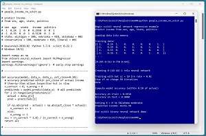 [Click on image for larger view.] Figure 1: Regression Using a scikit Neural Network
After training, the model is applied to the training data and the test data. The model scores 91.50 percent accuracy (183 out of 200 correct) on the training data, and 90.00 percent accuracy (36 out of 40 correct) on the test data. The demo program defines a correct income prediction as one that's within 10 percent of the true income.
The demo concludes by predicting the income of a new, previously unseen person who is male, age 34, from Oklahoma, and who is a political moderate. The predicted income is $44,355.38.
This article assumes you have intermediate or better skill with a C-family programming language, but doesn't assume you know much about neural networks or the scikit library. The complete source code for the demo program is presented in this article and in the accompanying file download. The source code and data are also available online.
Installing the scikit Library
There are several ways to install the scikit library. I recommend installing the Anaconda Python distribution. Anaconda contains a core Python engine plus over 500 libraries that are (mostly) compatible with one another. I used Anaconda3-2020.02, which contains Python 3.7.6 and the scikit 0.22.1 version. The demo code runs on Windows 10 or 11.
Briefly, Anaconda is installed using a Windows self-extracting executable file. The setup process is mostly straightforward and takes about 15 minutes. You can follow these step-by-step instructions to help.
There are more up-to-date versions of Anaconda / Python / scikit library available. But because the Python ecosystem has hundreds of libraries, if you install the most recent versions of these libraries, you run a greater risk of library incompatibilities -- a major headache when working with Python.
The Data
The data is artificial. There are 200 training items and 40 test items. The structure of data looks like:
 1   0.24   1 0 0   0.2950   0 0 1
-1   0.39   0 0 1   0.5120   0 1 0
 1   0.63   0 1 0   0.7580   1 0 0
-1   0.36   1 0 0   0.4450   0 1 0
 1   0.27   0 1 0   0.2860   0 0 1
. . .
The tab-delimited fields are sex (-1 = male, 1 = female), age (divided by 100), state (Michigan = 100, Nebraska = 010, Oklahoma = 001), income (divided by $100,000) and political leaning (conservative = 100, moderate = 010, liberal = 001).
The numeric predictors should be normalized to all the same range -- typically 0.0 to 1.0 or -1.0 to +1.0 -- as normalizing prevents predictors with large magnitudes from overwhelming those with small magnitudes.
For categorical predictor variables, I recommend one-hot encoding. For example, if there were five states instead of just three, the states would be encoded as 10000, 01000, 00100, 00010, 00001.
For binary predictor variables, such as sex, you can encode using either zero-one encoding or minus-one-plus-one encoding. The demo uses minus-one-plus-one encoding. In spite of decades of research, there are some topics, such as binary predictor encoding, that are not well understood (see "Encoding Binary Predictor Variables for Neural Networks").
The Demo Program
The complete demo program is presented in Listing 1. Notepad is my preferred code editor but most of my colleagues prefer one of the many excellent IDEs that are available for Python. I indent my Python program using two spaces rather than the more common four spaces.
The program imports the NumPy library, which contains numeric array functionality, and the MLPRegressor module, which contains neural network functionality. Notice the name of the root scikit module is sklearn rather than scikit.
import numpy as np
from sklearn.neural_network import MLPRegressor
import warnings
warnings.filterwarnings('ignore')  # early-stop warnings
The demo specifies that no Python warnings should be displayed. I do this to keep the output tidy, but in a non-demo scenario you definitely want to see warning messages.
Listing 1: Complete Demo Program
# people_income_nn_sckit.py

# predict income
# from sex, age, state, politics

# sex  age   state   income  politics
#  1  0.24  1  0  0  0.2950  0  0  1
# -1  0.39  0  0  1  0.5120  0  1  0
# state: michigan = 100, nebraska = 010, oklahoma = 001
# conservative = 100, moderate = 010, liberal = 001

# Anaconda3-2020.02  Python 3.7.6  scikit 0.22.1
# Windows 10/11

import numpy as np
from sklearn.neural_network import MLPRegressor
import warnings
warnings.filterwarnings('ignore')  # early-stop warnings

# ---------------------------------------------------------

def accuracy(model, data_x, data_y, pct_close=0.10):
  # accuracy predicted within pct_close of actual income
  # item-by-item allows inspection but is slow
  n_correct = 0; n_wrong = 0
  predicteds = model.predict(data_x)  # all predicteds
  for i in range(len(predicteds)):
    actual = data_y[i]
    pred = predicteds[i]

    if np.abs(pred - actual) < np.abs(pct_close * actual):
      n_correct += 1
    else:
      n_wrong += 1
  acc = (n_correct * 1.0) / (n_correct + n_wrong)
  return acc

# ---------------------------------------------------------

def accuracy_q(model, data_x, data_y, pct_close=0.10):
  # accuracy within pct_close of actual income
  # all-at-once is quick
  n_items = len(data_y)
  preds = model.predict(data_x)  # all predicteds

  n_correct = np.sum((np.abs(preds - data_y) < \
    np.abs(pct_close * data_y)))
  result = (n_correct / n_items)
  return result

# ---------------------------------------------------------

def main():
  # 0. get ready
  print("\nBegin scikit neural network regression example ")
  print("Predict income from sex, age, State, politics ")
  np.random.seed(1)
  np.set_printoptions(precision=4, suppress=True)

  # 1. load data
  print("\nLoading data into memory ")
  train_file = ".\\Data\\people_train.txt"
  train_xy = np.loadtxt(train_file, usecols=range(0,9),
    delimiter="\t", comments="#",  dtype=np.float32)
  train_x = train_xy[:,[0,1,2,3,4,6,7,8]]
  train_y = train_xy[:,5]

  test_file = ".\\Data\\people_test.txt"
  test_xy = np.loadtxt(test_file, usecols=range(0,9),
    delimiter="\t", comments="#",  dtype=np.float32)
  test_x = test_xy[:,[0,1,2,3,4,6,7,8]]
  test_y = test_xy[:,5]

  print("\nTraining data:")
  print(train_x[0:4])
  print(". . . \n")
  print(train_y[0:4])
  print(". . . ")

# ---------------------------------------------------------

  # 2. create network
  # MLPRegressor(hidden_layer_sizes=(100,),
  #  activation='relu', *, solver='adam', alpha=0.0001,
  #  batch_size='auto', learning_rate='constant',
  #  learning_rate_init=0.001, power_t=0.5, max_iter=200,
  #  shuffle=True, random_state=None, tol=0.0001,
  #  verbose=False, warm_start=False, momentum=0.9,
  #  nesterovs_momentum=True, early_stopping=False,
  #  validation_fraction=0.1, beta_1=0.9, beta_2=0.999,
  #  epsilon=1e-08, n_iter_no_change=10, max_fun=15000)

  params = { 'hidden_layer_sizes' : [10,10],
    'activation' : 'relu',
    'solver' : 'adam',
    'alpha' : 0.0,
    'batch_size' : 10,
    'random_state' : 0,
    'tol' : 0.0001,
    'nesterovs_momentum' : False,
    'learning_rate' : 'constant',
    'learning_rate_init' : 0.01,
    'max_iter' : 1000,
    'shuffle' : True,
    'n_iter_no_change' : 50,
    'verbose' : False }

  print("\nCreating 8-(10-10)-1 relu neural network ")
  net = MLPRegressor(**params)

# ---------------------------------------------------------

  # 3. train
  print("\nTraining with bat sz = " + \
    str(params['batch_size']) + " lrn rate = " + \
    str(params['learning_rate_init']) + " ")
  print("Stop if no change " + \
    str(params['n_iter_no_change']) + " iterations ")
  net.fit(train_x, train_y)
  print("Done ")

# ---------------------------------------------------------

  # 4. evaluate model
  # score() is coefficient of determination for MLPRegressor
  print("\nCompute model accuracy (within 0.10 of actual) ")
  acc_train = accuracy(net, train_x, train_y, 0.10)
  print("\nAccuracy on train = %0.4f " % acc_train)
  acc_test = accuracy(net, test_x, test_y, 0.10)
  print("Accuracy on test = %0.4f " % acc_test)

  # print("\nModel accuracy quick (within 0.10 of actual) ")
  # acc_train = accuracy_q(net, train_x, train_y, 0.10)
  # print("\nAccuracy on train = %0.4f " % acc_train)
  # acc_test = accuracy_q(net, test_x, test_y, 0.10)
  # print("Accuracy on test = %0.4f " % acc_test)

# ---------------------------------------------------------

  # 5. use model
  # no proba() for MLPRegressor
  print("\nSetting X = M 34 Oklahoma moderate: ")
  X = np.array([[-1, 0.34, 0,0,1,  0,1,0]])
  income = net.predict(X)  # divided by 100,000
  income *= 100000  # denormalize
  print("Predicted income: %0.2f " % income)

# ---------------------------------------------------------

  # 6. TODO: save model using pickle

  print("\nEnd scikit binary neural network demo ")

if __name__ == "__main__":
  main()
All the program logic is contained in a main() function. The demo defines an accuracy() function that optimizes clarity at the expense of speed and a second accuracy_q() function (the "q" means "quick") that optimizes performance. The demo begins by setting the NumPy random seed:
def main():
  # 0. get ready
  print("Begin scikit neural network regression example ")
  print("Predict income from sex, age, State, politics ")
  np.random.seed(1)
  np.set_printoptions(precision=4, suppress=True)
 . . .
Technically, setting the random seed value isn't necessary, but doing so helps you to get reproducible results in most situations. The set_printoptions() function formats NumPy arrays to four decimals without using scientific notation.
Loading the Training and Test Data
The demo program loads the training data into memory using these statements:
  # 1. load data
  print("Loading data into memory ")
  train_file = ".\\Data\\people_train.txt"
  train_xy = np.loadtxt(train_file, usecols=range(0,9),
    delimiter="\t", comments="#",  dtype=np.float32)
  train_x = train_xy[:,[0,1,2,3,4,6,7,8]]
  train_y = train_xy[:,5]
This code assumes the data files are stored in a directory named Data. There are many ways to load data into memory. I prefer using the NumPy library loadtxt() function but a common alternative is the Pandas library read_csv() function.
The code reads all 200 lines of training data (columns 0 to 8 inclusive) into a matrix named train_xy and then splits the data into a matrix of predictor values and a vector of target income values. The colon syntax means "all rows."
The 40-item test data is read into memory in the same way as the training data:
  test_file = ".\\Data\\people_test.txt"
  test_xy = np.loadtxt(test_file, usecols=range(0,9),
    delimiter="\t", comments="#",  dtype=np.float32)
  test_x = test_xy[:,[0,1,2,3,4,6,7,8]]
  test_y = test_xy[:,5]
The demo program prints the first four predictor items and the first four target politics values:
  print("Training data:")
  print(train_x[0:4])
  print(". . . ")
  print(train_y[0:4])
  print(". . . ")
In a non-demo scenario you might want to display all the training data and all the test data to verify the data has been read properly.
Creating the Neural Network Model
Creating the multi-class classification neural network model is simultaneously simple and complicated. First, the demo program sets up the network parameters in a Python Dictionary object like so:
  # 2. create network
  params = { 'hidden_layer_sizes' : [10,10],
    'activation' : 'relu', 'solver' : 'adam',
    'alpha' : 0.0, 'batch_size' : 10,
    'random_state' : 0, 'tol' : 0.0001,
    'nesterovs_momentum' : False,
    'learning_rate' : 'constant',
    'learning_rate_init' : 0.01,
    'max_iter' : 1000, 'shuffle' : True,
    'n_iter_no_change' : 50, 'verbose' : False }
After the parameters are set, they are fed to a neural network constructor:
  print("Creating 8-(10-10)-1 relu neural network ")
  net = MLPRegressor(**params)
The ** syntax means to unpack the Dictionary values and pass them to the constructor. Like many scikit models, the MLPClassifier class has a lot of parameters and default values. The constructor signature is:
MLPRegressor(hidden_layer_sizes=(100,),
  activation='relu', *, solver='adam', alpha=0.0001,
  batch_size='auto', learning_rate='constant',
  learning_rate_init=0.001, power_t=0.5, max_iter=200,
  shuffle=True, random_state=None, tol=0.0001,
  verbose=False, warm_start=False, momentum=0.9,
  nesterovs_momentum=True, early_stopping=False,
  validation_fraction=0.1, beta_1=0.9, beta_2=0.999,
  epsilon=1e-08, n_iter_no_change=10, max_fun=15000)
When working with scikit, you'll spend most of your time reading the documentation and trying to figure out what each parameter does. The MLPRegressor class is especially complex because many of the parameters interact with one another.
Your first parameter decision is the solver to use for training the network. Your choices are 'adam', 'sgd', or 'lbfgs'. I recommend 'sgd' for most problems, even though 'adam' is the default. The 'adam' solver is essentially a sophisticated version of 'sgd'. The 'lbfgs' solver works in a completely different way from 'adam' and 'sgd'. The demo program uses 'adam' optimization only because it gave better results than 'sgd' optimization.
Your next parameter decision is the number of hidden layers and the number of processing nodes in each layer. The demo uses two hidden layers with 10 nodes each. More layers and more nodes are not always better, so you must experiment. The default is one hidden layer with 100 nodes.
Your next decision is hidden node activation. Your choices are 'identity', 'logistic', 'tanh', 'relu'. If you use an 'sgd' solver' I suggest trying 'tanh' activation first. If you use an 'adam' solver', I suggest trying 'relu' activation first. The demo uses 'relu' activation. The 'identity' and 'logistic' hidden node activation are rarely used.
Your next set of decisions are related to the training learning rate. The demo uses the 'constant' rate type. Alternatives are 'invscaling' and 'adaptive'. These are very complicated and I don't recommend using them. If you use a 'constant' learning rate type, you specify that rate using the learning_rate_init parameter. This value often has a huge effect on the performance of the resulting neural network model. Typical values to experiment with are 0.001, 0.01, 0.05 and 0.10. The demo uses a 0.01 learning rate.
Your next decision is the batch_size parameter. The demo uses 10. I recommend that your batch size evenly divide the number of training items so that all batches of training data have the same size. Because the demo has 200 training items, each batch will have 200 / 10 = 20 data items.
Your next parameter decision is whether or not to use nesterovs_momentum. The default value is True, but I recommend setting to False. Momentum is an old technique that was designed primarily to speed up training. But the advantage gained by using momentum is outweighed, in my opinion, by having to experiment with yet another parameter value, the momentum parameter.
Your next parameter decision is the alpha value. The alpha parameter controls what is called L2 regularization. Regularization shrinks the weights and biases of neural network to prevent them from becoming huge, which in turn can cause model overfitting. Overfitting means the model predicts well on the training data, but when presented with new, previously unseen test data, the model predicts poorly. The default value of alpha is 0.0001, but I recommend setting alpha to zero and only experimenting with alpha values if severe overfitting occurs.
Your next parameter decision is max_iter to set the maximum number of training iterations. The demo sets max_iter to 1000. This is strictly a matter of trial and error. The demo sets the verbose parameter to False, but setting it to True will allow you to monitor training and determine a good value for the max_iter parameter (when the loss value stops changing much).
Your last parameter decisions are n_iter_no_change and tol. The n_iter_no_change specifies that training should stop if there are a certain number of iterations where no improvement (decrease in the error/loss value) has been made. The tol ("tolerance") parameter specifies exactly what no improvement means.
To recap, the MLPRegressor has a large number of interacting parameters. There are essentially an infinite number of combinations of the values of the parameters, so you must experiment using trial and error. With each neural network example you encounter, your intuition will grow, and you'll be able to zero-in on good parameters values more quickly. This is the reason that machine learning with neural networks is sometimes said to be part art and part science.
Training the Neural Network
After the neural network has been prepared, training is easy:
  # 3. train
  print("Training with bat sz = " + \
    str(params['batch_size']) + " lrn rate = " + \
    str(params['learning_rate_init']) + " ")
  print("Stop if no change " + \
    str(params['n_iter_no_change']) + " iterations ")
  net.fit(train_x, train_y)
  print("Done ")
The backslash character is used for Python line continuation. The fit() method requires a matrix of predictor values and a vector of target labels. There are no optional parameters for fit() so you don't have much to think about -- all the decisions are made when you set the MLPRegressor constructor parameters.
Evaluating the Trained Model
The demo computes the accuracy of the trained model like so:
  # 4. evaluate model
  print("Compute model accuracy (within 0.10 of actual) ")
  acc_train = accuracy(net, train_x, train_y, 0.10)
  print("Accuracy on train = %0.4f " % acc_train)
  acc_test = accuracy(net, test_x, test_y, 0.10)
  print("Accuracy on test = %0.4f " % acc_test)
For most scikit classifiers, the built-in score() function computes a simple accuracy which is just the number of correct predictions divided by the total number of predictions. But for an MLPRegressor network you must define what a correct prediction is and write a program-defined custom accuracy function. The demo defines a correct income prediction as one that is within a specified percentage of the true target income value. The key statement is:
if np.abs(pred - actual) < np.abs(pct_close * actual):
  n_correct += 1
else:
  n_wrong += 1
The demo program defines two different accuracy functions. The first accuracy function iterates through each prediction one at a time. This approach allows you to insert diagnostic print() statements to investigate incorrect predictions, but iterating is slow.
The second accuracy function uses a set approach instead of iteration. This accuracy function is faster but you can't easily examine incorrect predictions.
Using the Trained Model
The demo uses the trained model like so:
  # 5. use model
  print("Setting X = M 34 Oklahoma moderate: ")
  X = np.array([[-1, 0.34, 0,0,1,  0,1,0]])
  income = net.predict(X)  # divided by 100,000
  income *= 100000  # denormalize
  print("Predicted income: %0.2f " % income)
Because the neural network model was trained using normalized and encoded data, the X-input must be normalized and encoded in the same way. Notice the double square brackets on the X-input. The predict() method expects a matrix rather than a vector. The predicted income value is normalized so the demo multiplies the prediction by 100,000 to make the result easier to read.
In most situations you will want to save the trained regression model so that it can be used by other programs. There are several ways to save a scikit model, but using the pickle library ("pickle" means to preserve in ordinary English) is the simplest and most common. For example:
print("Saving trained network ")
path = ".\\Models\\people_income_net.sav"
pickle.dump(model, open(path, "wb"))
This code assumes there is a subdirectory named Models. The saved model can be loaded into memory and used like this:
X = np.array([[-1, 0.34, 0,0,1,  0,1,0]]], dtype=np.float32)
with open(path, 'rb') as f:
  loaded_model = pickle.load(f)
inc = loaded_model.predict(X)
Wrapping Up
The scikit MLPRegressor neural network module is the most powerful scikit technique for regression problems, but the technique requires lots of labeled training data (typically at least 100 items). For situations where you don't have lots of training data, alternatives include the scikit Ridge Regression, Kernel Ridge Regression and Lasso Regression modules.