The Data Science Lab

Gaussian Naive Bayes Classification Using the scikit Library

Dr. James McCaffrey of Microsoft Research says the main advantage of using Gaussian naive Bayes classification compared to other techniques like decision trees or neural networks is that you don't have to fine-tune model parameters.

• By James McCaffrey
• 05/31/2023

Gaussian naive Bayes classification is a classical machine learning technique that can be used to predict a discrete value when the predictor variables are all numeric. For example, you might want to predict a person's political leaning (conservative, moderate, liberal) from their age, annual income and bank account balance.

There are several other variations of naive Bayes (NB) classification including Categorical NB, Bernoulli NB, and Multinomial NB. The different NB variations are used for different types of predictor data. In Categorical NB the predictor values are strings like "red," "blue" and "green." In Bernoulli NB the predictor values are Boolean/binary like "male" and "female." In Multinomial NB the predictor values are integer counts.

This article explains Gaussian NB classification by presenting an end-to-end demo. The goal of the demo is to predict the species of a wheat seed (Kama = 0, Rosa = 1, Canadian = 2) from seven numeric predictor variables: seed length, width, perimeter and so on.

There are several tools and code libraries that you can use to perform Gaussian NB classification. The scikit-learn library (also called scikit or sklearn) is based on the Python language and is one of the most popular machine learning libraries.

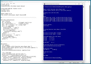
A good way to see where this article is headed is to take a look at the screenshot in Figure 1. The demo program begins by loading a 180-item set of training data and a 30-item set of test data into memory. The data is normalized so that all predictor values are between 0.0 and 1.0. The demo creates a Gaussian NB prediction model. The model scores 93.33 percent accuracy on the training data (168 out of 180 correct) and 66.67 percent accuracy on the test data (20 out of 30 correct).

The demo computes and displays a confusion matrix for the test data that shows how the prediction model performs for each of the three class labels / species. The model predicts wheat species Canadian quite well (9 out of 10 correct), but predicts species Rosa poorly (only 5 out of 10 correct).

The demo concludes by predicting the species of a dummy wheat seed that has all predictor values set to 0.2. The predicted pseudo-probabilities for each species are [0.0033, 0.0000, 0.9667]. Because the pseudo-probability at index [2] is the largest, the predicted species is 2 = Canadian.

This article assumes you have intermediate or better skill with a C-family programming language such as Python or C#, but doesn't assume you know much about Gaussian naive Bayes classification or the scikit library. The complete source code for the demo program is presented in this article. The source code is also available in the accompanying file download and is also online.

Installing the scikit Library
There are several ways to install the scikit library. I recommend installing the Anaconda Python distribution, which contains scikit and core Python engine, plus more than 500 libraries that are (mostly) compatible with one another. I used Anaconda3-2022.10, which contains Python 3.9.13 and the scikit 1.0.2 version. The code presented here works on earlier versions of Python and scikit too. The demo code runs on Windows 10 or 11.

Briefly, Anaconda is installed using a Windows self-extracting executable file. The setup process is mostly straightforward and takes about 15 minutes following step-by-step instructions. The instructions can be easily adapted for Anaconda3-2022-10 with Python 3.9.13.

There are more up-to-date versions of Anaconda / Python / scikit library available. However, because the Python ecosystem has hundreds of libraries, if you install the most recent versions of these libraries, you run a greater risk of library incompatibilities -- a standard headache when working with Python.

The Data
The Wheat Seeds dataset has 210 items. The raw data looks like:

15.26  14.84  0.871   5.763  3.312  2.221  5.22   1
14.88  14.57  0.8811  5.554  3.333  1.018  4.956  1
. . .
17.63  15.98  0.8673  6.191  3.561  4.076  6.06   2
16.84  15.67  0.8623  5.998  3.484  4.675  5.877  2
. . .
11.84  13.21  0.8521  5.175  2.836  3.598  5.044  3
12.3   13.34  0.8684  5.243  2.974  5.637  5.063  3

Each line of data represents a wheat seed. The first seven values on each line are the predictor values: seed area, perimeter, compactness, length, width, asymmetry, groove. The last value on each line is the species: Kama = 1, Rosa = 2, Canadian = 3.

It's not necessary to normalize predictor values when using Gaussian NB classification, but normalization doesn't hurt and normalized data can be used by other techniques, such as a neural network, that need normalization. So I normalized the data.

I divided each predictor column by a constant: (25, 20, 1, 10, 10, 10, 10) respectively. The resulting predictors are all between 0.0 and 1.0. I also re-coded the target class labels from 1-based to 0-based. The resulting 210-item normalized and encoded data looks like:

0.6104  0.7420  0.8710  0.5763  0.3312  0.2221  0.5220  0
0.5952  0.7285  0.8811  0.5554  0.3333  0.1018  0.4956  0
. . .
0.7052  0.7990  0.8673  0.6191  0.3561  0.4076  0.6060  1
0.6736  0.7835  0.8623  0.5998  0.3484  0.4675  0.5877  1
. . .
0.5048  0.6835  0.8481  0.5410  0.2911  0.3306  0.5231  2
0.5104  0.6690  0.8964  0.5073  0.3155  0.2828  0.4830  2

I split the 210-item normalized data into a 180-item training set and a 30-item test set. I used the first 60 of each target class for training and the last 10 of each target class for testing using training and test data.

Understanding How Gaussian Naive Bayes Classification Works
Understanding how Gaussian naive Bayes classification works is best explained by example. Suppose, as in the demo program, the goal is to predict wheat seed species from seven predictor variables, and the item-to-predict has normalized values [0.1, 0.2, 0.3, 0.4, 0.5, 0.6, 0.7].

Gaussian NB examines each predictor variable separately. Suppose in the training data that the average value in column 1 (seed area) for class 0 is 0.6, the average value for class 1 is 0.8 and the average value for class 2 is 0.3. Based on this limited information looking at just the first predictor, you'd guess that the unknown item is class 2 because the unknown predictor value of 0.1 is closest to the average value for class 2 of 0.3.

Now you could examine each of the other six predictors. Suppose they suggest that the class of the unknown item is 1, 2, 2, 0, 2, 2 respectively. At this point, five of the seven predictor values suggest that the class of the unknown item is class 2, one predictor suggests class 0, and one predictor suggests class 1. You could use a majority-rule approach and conclude that the unknown item is class 2. However, a majority-rule approach doesn't take into account the strength of each of the seven guesses. Gaussian naive Bayes uses Bayesian mathematics to combine the evidence values to produce a final prediction in the form of pseudo-probabilities.

Gaussian NB is called "naive" (meaning unsophisticated) because each predictor variable is analyzed independently, not taking into account interactions between variables. The technique is called Gaussian because it assumes that each predictor variable is Gaussian (bell-shaped) distributed. The name "Bayes" refers to Thomas Bayes (1701-1761), a founder of probability theory.

The Demo Program
The complete demo program is presented in Listing 1. I am a proud user of Notepad as my preferred code editor, but most of my colleagues use something more sophisticated. I indent my Python program using two spaces rather than the more common four spaces.

The program imports the NumPy library, which contains numeric array functionality. The GaussianNB module has the key code for performing Gaussian naive Bayes classification. Notice the name of the root scikit module is sklearn rather than scikit.

# wheat_gnb.py
# Gaussian NB on the Wheat Seeds dataset

# Anaconda3-2022.10  Python 3.9.13
# scikit 1.0.2  Windows 10/11 

import numpy as np
from sklearn.naive_bayes import GaussianNB

# ---------------------------------------------------------

def show_confusion(cm):
  dim = len(cm)
  mx = np.max(cm)             # largest count in cm
  wid = len(str(mx)) + 1      # width to print
  fmt = "%" + str(wid) + "d"  # like "%3d"
  for i in range(dim):
    print("actual   ", end="")
    print("%3d:" % i, end="")
    for j in range(dim):
      print(fmt % cm[i][j], end="")
    print("")
  print("------------")
  print("predicted    ", end="")
  for j in range(dim):
    print(fmt % j, end="")
  print("")

# ---------------------------------------------------------

def main():
  # 0. prepare
  print("\nBegin scikit Gaussian naive Bayes demo ")
  print("Predict wheat species (0,1,2) from seven numerics ")
  np.random.seed(1)
  np.set_printoptions(precision=4, suppress=True)

  # 1. load data
  print("\nLoading train and test data ")
  train_file = ".\\Data\\wheat_train_k.txt"
  x_train = np.loadtxt(train_file, usecols=[0,1,2,3,4,5,6],
    delimiter="\t", comments="#", dtype=np.float32)
  y_train = np.loadtxt(train_file, usecols=7,
    delimiter="\t", comments="#", dtype=np.int64) 

  test_file = ".\\Data\\wheat_test_k.txt"
  x_test = np.loadtxt(test_file, usecols=[0,1,2,3,4,5,6],
    delimiter="\t", comments="#", dtype=np.float32)
  y_test = np.loadtxt(test_file, usecols=7,
    delimiter="\t", comments="#", dtype=np.int64) 
  print("Done ")

  print("\nData: ")
  print(x_train[0:4][:])
  print(". . .")
  print("\nActual species: ")
  print(y_train[0:4])
  print(". . .")

  # 2. create and train model
  # GaussianNB(*, priors=None, var_smoothing=1e-09)
  print("\nCreating Gaussian naive Bayes classifier ")
  model = GaussianNB()
  model.fit(x_train, y_train)
  print("Done ")

  # 3. evaluate model
  acc_train = model.score(x_train, y_train)
  print("\nAccuracy on train data = %0.4f " % acc_train)
  acc_test = model.score(x_test, y_test)
  print("Accuracy on test data =  %0.4f " % acc_test)

  # 3b. confusion matrix
  from sklearn.metrics import confusion_matrix
  y_predicteds = model.predict(x_test)
  cm = confusion_matrix(y_test, y_predicteds) 
  print("\nConfusion matrix for test data: ")
  show_confusion(cm)

  # 4. use model
  print("\nPredicting species all 0.2 predictors: ")
  X = np.array([[0.2, 0.2, 0.2, 0.2, 0.2, 0.2, 0.2]],
    dtype=np.float32)
  print(X)
  probs = model.predict_proba(X)
  print("\nPrediction probs: ")
  print(probs)

  predicted = model.predict(X)
  print("\nPredicted class: ")
  print(predicted)

  # 5. TODO: save model using pickle
  
  print("\nEnd demo ")

if __name__ == "__main__":
  main()

The demo begins by setting the NumPy random seed:

def main():
  # 0. prepare
  print("Begin scikit Gaussian naive Bayes demo ")
  print("Predict wheat species (0,1,2) from seven numerics ")
  np.random.seed(1)
  np.set_printoptions(precision=4, suppress=True)
. . .

Technically, setting the random seed value isn't necessary, but doing so allows you to get reproducible results in most situations.

Loading the Training and Test Data
The demo program loads the training data into memory using these statements:

  # 1. load data
  print("Loading train and test data ")
  train_file = ".\\Data\\wheat_train_k.txt"
  x_train = np.loadtxt(train_file, usecols=[0,1,2,3,4,5,6],
    delimiter="\t", comments="#", dtype=np.float32)
  y_train = np.loadtxt(train_file, usecols=7,
    delimiter="\t", comments="#", dtype=np.int64)

This code assumes the data files are stored in a directory named Data. There are many ways to load data into memory. I prefer using the NumPy library loadtxt() function, but common alternatives are the NumPy genfromtxt() function and the Pandas library read_csv() function.

The demo reads the 180-item training predictors and the target class labels using two calls to the loadtxt() function. An alternative technique is to read all the data into a single matrix and then split the data into a matrix of predictor values and a vector of target labels.

The demo loads the 30-item test data similarly:

  test_file = ".\\Data\\wheat_test_k.txt"
  x_test = np.loadtxt(test_file, usecols=[0,1,2,3,4,5,6],
    delimiter="\t", comments="#", dtype=np.float32)
  y_test = np.loadtxt(test_file, usecols=7,
    delimiter="\t", comments="#", dtype=np.int64) 
  print("Done ")

The demo program shows the first four training items and their associated target labels:

  print("Data: ")
  print(x_train[0:4][:])
  print(". . .")
  print("Actual species: ")
  print(y_train[0:4])
  print(". . .")

In a non-demo scenario, you might want to display all of the training data.

Creating and Training the Model
Creating and training the Gaussian naive Bayes classification model is simple:

  # 2. create and train model
  print("Creating Gaussian naive Bayes classifier ")
  model = GaussianNB()
  model.fit(x_train, y_train)
  print("Done ")

Unlike many scikit models, the GaussianlNB class has relatively few (just two) parameters. The constructor signature is:

GaussianNB(*, priors=None, var_smoothing=1e-09)

When working with scikit, you'll spend most of your time reading the documentation and trying to figure out what each model parameter does. The priors parameter allows you to specify the initial probabilities of each target class. For example, for the demo training data there are 60 items of each of the three classes/species, and so the GaussianNB algorithm uses prior probabilities of 0.3333 for each class. If you passed [0.25, 0.50, 0.25] to the GaussianNB constructor, the algorithm would use those values for initial probabilities. The priors parameter is typically used when you have limited data in one target class and you want to specify equal initial probabilities.

The var_smoothing parameter adds a value to all predictor variances. The value added is a proportion of the largest predictor variance. The idea is that predictors with small variances can overwhelm predictors with large variances (because a predictor's variance appears in a fraction denominator during calculations). Adding a var_smoothing factor can artificially increase small variances to prevent a small-variance predictor from dominating the overall pseudo-probability calculations. In practice, the var_smoothing parameter is rarely used.

Evaluating the Trained Model
The demo computes the accuracy of the trained model like so:

  # 3. evaluate model
  acc_train = model.score(x_train, y_train)
  print("Accuracy on train data = %0.4f " % acc_train)
  acc_test = model.score(x_test, y_test)
  print("Accuracy on test data =  %0.4f " % acc_test)

The score() function computes a simple accuracy, which is just the number of correct predictions divided by the total number of predictions. However, for classification problems you usually want additional evaluation metrics to show how the model predicts for different target labels. For example, if a 100-item training dataset had 95 Kama seeds, 3 Rosa seeds and 2 Canadian seeds, then predicting Kama for any input would score 95 percent accuracy.

The scikit library has many ways to evaluate a trained classification prediction model. A good technique is to compute and display a confusion matrix:

  # 3b. confusion matrix
  from sklearn.metrics import confusion_matrix
  y_predicteds = model.predict(x_test)
  cm = confusion_matrix(y_test, y_predicteds) 
  print("Confusion matrix for test data: ")
  # print(cm)  # raw 
  show_confusion(cm)  # formatted

For the demo training data, the output of a raw confusion matrix would be:

[[6 0 4]
 [5 5 0]
 [1 0 9]]

A raw scikit confusion matrix is difficult to interpret so I usually implement a program-defined function called show_confusion() that adds basic labels. The output of show_confusion() is:

actual     0: 6 0 4
actual     1: 5 5 0
actual     2: 1 0 9
------------
predicted     0 1 2

The formatted output is much easier to interpret than the raw output. You can find the source code for the show_confusion() function in Listing 1.

Using the Trained Model
The demo program uses the model to predict the course type of a new, previously unseen dummy wheat seed:

  # 4. use model
  print("Predicting species all 0.2 predictors: ")
  X = np.array([[0.2, 0.2, 0.2, 0.2, 0.2, 0.2, 0.2]],
    dtype=np.float32)
  print(X)
  probs = model.predict_proba(X)
  print("Prediction probs: ")
  print(probs)

Notice the double square brackets on the x-input. The predict_proba() function expects a matrix rather than a vector. Because the GaussianNB model was trained using normalized data, the seven input values must be normalized in the same way, by dividing raw values by (25, 20, 1, 10, 10, 10, 10) respectively.

The return result from the predict_proba() function ("probabilities array") for the demo data is [[0.0033, 0.0000, 0.9967 ]]. The result has only one row because only one input was supplied. The three values in the row are the pseudo-probabilities of class 0, 1, and 2 respectively.

The demo program concludes with:

  predicted = model.predict(X)
  print("Predicted class: ")
  print(predicted)

  # 5. TODO: save model using pickle
  print("End demo ")
if __name__ == "__main__":
  main()

The predict() method returns the predicted class, 0, 1, 2, rather than pseudo-probabilities.

Saving the Trained Model
The demo doesn't save the trained model. When using scikit, the most common way to save a trained naive Bayes classifier model is to use the pickle library ("pickle" means to preserve in English, as in "pickled cucumbers"). For example:

  import pickle
  print("Saving Gaussian naive Bayes model ")
  path = ".\\Models\\wheat_gnb_model.sav"
  pickle.dump(model, open(path, "wb"))

This code assumes there is a directory named Models. The saved model could be loaded and used from another program like so:

  # predict for unknown wheat seed
  X = np.array([[0.1, 0.2, 0.3, 0.4, 0.5, 0.6, 0.7]],
    dtype=np.float32)
  with open(path, 'rb') as f:
    loaded_model = pickle.load(f)
  pa = loaded_model.predict_proba(x)
  print(pa)  # pseudo-probabilities

There are several other ways to save and load a trained scikit model, but using the pickle library is simplest.

Wrapping Up
The main advantage of using Gaussian naive Bayes classification compared to other techniques like decision trees or neural networks is that you don't have to fine-tune model parameters. The main disadvantage of Gaussian NB is that the technique assumes all predictor variables are Gaussian distributed, which is often not true, and therefore the technique is typically not as powerful as a well-tuned decision tree or neural network model. Another disadvantage is that Gaussian NB requires all predictors to be numeric and so it can't handle categorical predictors (like color = "red", "blue", or "green") or Boolean predictors (like a person's sex = male or female).

Because Gaussian naive Bayes classification is so easy to use, my colleagues and I often use the technique to establish a baseline accuracy. Then a more powerful model, usually a neural network classifier, can be constructed with a rough idea of how accurate the model should be.

• Get Code Download