The Data Science Lab
Nadaraya-Watson Kernel Regression Using C#
The goal of a machine learning regression problem is to predict a single numeric value. For example, you might want to predict a person's income based on their age, height, high school GPA, and so on. There are approximately a dozen common regression techniques, including ordinary linear regression, k-nearest neighbors regression, random forest regression, kernel ridge regression, and neural network regression.
There are several versions of kernel regression, and each version has several variations. The specific type of kernel regression presented in this article is Nadaraya-Watson kernel regression using a radial basis function kernel. The term "kernel regression" by itself is ambiguous because there are many techniques that are called kernel regression in a given context. For example, kernel ridge regression (KRR) is very different from the technique presented in this article, but KRR is often shortened to just "kernel regression". Because of the possible naming confusion, I'll use the term NW kernel regression.
A good way to see where this article is headed is to take a look at the screenshot in Figure 1. The demo program begins by loading synthetic training and test data into memory. The data looks like:
-0.1660,  0.4406, -0.9998, -0.3953, -0.7065,  0.4840
 0.0776, -0.1616,  0.3704, -0.5911,  0.7562,  0.1568
-0.9452,  0.3409, -0.1654,  0.1174, -0.7192,  0.8054
 0.9365, -0.3732,  0.3846,  0.7528,  0.7892,  0.1345
. . .
There are 200 training items and 40 test items. The first five values on each line are the x predictors. The last value on each line is the target y variable to predict. The demo creates a NW kernel regression model, evaluates the model, and uses the model to make a prediction. The key lines of output are:
Creating NW kernel regressor with RBF gamma = 6.00
Done

Evaluating model
MSE train = 0.0140
MSE test = 0.0405
Accuracy train (within 0.10) = 0.9400
Accuracy test (within 0.10) = 0.6250

Predicting for x =
  -0.1660   0.4406  -0.9998  -0.3953  -0.7065
Predicted y = 0.5308
A NW kernel regression model requires a kernel function which measures the similarity between two data items. The demo uses a radial basis function (RBF) kernel. The RBF kernel requires a single parameter, gamma, which is set to 6.00 in the demo. The gamma parameter must be determined by trial and error.
Unlike many machine learning regression techniques, NW kernel regression does not do any explicit training to produce a mathematical prediction equation. NW kernel regression predictions are generated directly from the training data. This type of regression model is called nonparametric. In some sense, the training data is the model.
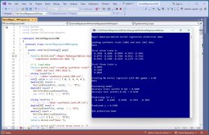 [Click on image for larger view.] Figure 1: Nadaraya-Watson Kernel Regression in Action
The demo computes the mean squared error of the NW regression model on the training data (MSE = 0.0140) and on the test data (MSE = 0.0405). Then the demo computes the accuracy of the model as 94.00% on the training data (188 out of 200 correct) and 62.50% on the test data (25 out of 40 correct). When using NW kernel regression, it's easy to get nearly perfect prediction accuracy on the training data. The challenge is to find a good value for the RBF gamma parameter that balances accuracy and error on the training and test data to avoid model overfitting.
The demo concludes by using the model to predict the target y for the first training item x = [-0.1660, 0.4406, -0.9998, -0.3953, -0.7065]. The predicted y is 0.5308 which is reasonably close to the true target y of 0.4840.
This article assumes you have intermediate or better programming skill but doesn't assume you know anything about NW kernel regression. The demo is implemented using C# but you should be able to refactor the demo code to another C-family language if you wish. All normal error checking has been removed to keep the main ideas as clear as possible.
The source code for the demo program is a bit too long to be presented in its entirety in this article. The complete code and data are available in the accompanying file download, and they're also available online.
The Demo Data
The demo data is synthetic. It was generated by a 5-10-1 neural network with random weights and bias values. The idea here is that the synthetic data does have an underlying, but complex, non-linear structure which can be predicted.
All of the predictor values are between -1 and +1. When using NW kernel regression, you must normalize/scale the predictor values to roughly the same range so that variables with large magnitudes (such as employee income) don't dominate variables with small magnitudes (such as high school GPA). The three most common normalization techniques are min-max, z-score, and divide-by-constant. When possible, I recommend using the divide-by-constant technique. For example, if you have a predictor variable employee age, you could divide all age values by 100.
NW kernel regression is most often used with data that has strictly numeric predictor variables. It is possible to use NW kernel regression with mixed categorical and numeric data, by using one-over-n-hot encoding on categorical data (such as a variable color with possible values red, blue, green), and equal interval encoding on data that has inherent ordering (such as a variable size with possible values small, medium, large).
Understanding the Radial Basis Function Kernel
In order to understand NW kernel regression, you must understand radial basis function (RBF) kernel functions. The RBF kernel computes a measure of similarity between two vectors. There are several RBF versions. The two most common are the sigma (bandwidth) and the gamma (inverse bandwidth) versions:
1.) rbf(x0, x1) = exp( -1 * ||x0 - x1||^2 / (2 * sigma^2) )
2.) rbf(x0, x1) = exp( -1 * gamma * ||x0 - x1||^2 )
Here, x0 and x1 are two vectors, exp() is the math e constant (2.71828...) raised to a power, ||x0 - x1||^2 is squared Euclidean distance, and sigma and gamma are arbitrary constants. The demo program uses the gamma version of RBF.
For example, if x0 = (2.50, -3.25, 1.20) and x1 = (2.0, -3.0, 1.0) and gamma = 0.25 then the squared Euclidean distance is sum of the squared differences between vector elements:
||x0 - x1||^2 = (2.50 - 2)^2 + (-3.25 - (-3))^2 + (1.20 - 1)^2
              = (0.50)^2 + (-0.25)^2 + (0.20)^2
              = 0.2500 + 0.0625 + 0.0400
              = 0.3525
and then RBF is:
rbf(x0, x1) = exp( -1  * gamma * ||x0 - x1||^2 )
            = exp( -0.25 * 0.3525 )
            = exp( -0.0881 )
            = 0.9156
If two vectors are the same, then rbf(x0, x1) = 1.0 (maximum similarity). As rbf(x0, x1) approaches but never quite reaches 0.0, it means the two vectors are less similar. RBF is symmetric so rbf(x0, x1) = rbf(x1, x0).
The RBF definition with sigma is the original form used in mathematics. The sigma constant is called the bandwidth of the RBF. But in machine learning, it's more common to use the RBF definition with gamma. Notice that gamma = 1 / (2 * sigma^2), or sigma = sqrt(1 / 2g). For the example vectors above, with gamma = 0.25, sigma = sqrt(1 / 0.50) = sqrt(2) = 1.414. If you use this value in the sigma version of the RBF definition, you will get the same 0.9156 result.
In math and research documentation, a general kernel function is sometimes written as K(x, x') to indicate any kernel function can be used and that x' is a reference (non-changing) vector. Sometimes kernel functions are defined so that they accept a just single vector, and you see K(x - x') to indicate you perform vector subtraction and then feed the result to the single-parameter kernel function.
Understanding Nadaraya-Watson Kernel Regression
The key equation for NW kernel regression is y(x) = Sum( K(x, xi) * yi ) / Sum( K(x, xi) ). Here x is an input vector, and y(x) is the predicted y value for x. The right side of the equation is a fraction. The top part is the sum of the kernel function applied to x and each training data item xi, times the corresponding yi value. The bottom part of the fraction is the same, but there's no multiplication by yi.
Suppose the x to predict is (2.0, 4.0, 1.0) and you have just three training data items, and you use the RBF kernel function with some value for gamma:
x0 = (3.0, 3.0, 2.0)  y0 = 0.7
x1 = (4.0, 1.0, 0.0)  y1 = 0.6
x2 = (2.0, 5.0, 1.0)  y2 = 0.8

rbf(x, x0) = 0.5
rbf(x, x1) = 0.4
rbf(x, x2) = 0.3
The top part of the prediction fraction is:
Sum( K(x, xi) * yi ) = [rbf(x, x0) * y0] +
                       [rbf(x, x1) * y1] +
                       [rbf(x, x2) * y2]
                     = (0.5 * 0.7) + (0.4 * 0.6) + (0.3 * 0.8)
                     = 0.35 + 0.24 + 0.24
                     = 0.83
The bottom part of the fraction is:
Sum( K(x, xi) ) = rbf(x, x0) + rbf(x, x1) + rbf(x, x2)
                = 0.5 + 0.4 + 0.3
                = 1.2
And the predicted y is:
y(x) = Sum( K(x, xi) * yi ) / Sum( K(x, xi) )
     = 0.83 / 1.2
     = 0.69
What is happening here is that a predicted y value is the weighted average of all the target y values in the training data, where the weights are the corresponding RBF kernel function values. When a kernel value is close to 1, it means the two vectors are similar and the predicted y component is close to the corresponding target y.
The Nadaraya-Watson technique is named after mathematicians Elizbar Nadaraya (Georgia) and Geoffrey Watson (Australia) who independently came up with the idea in 1964. The NW kernel regression technique is similar to weighted k-nearest neighbors regression, but instead of using just k training data items and Euclidean distance, NW kernel regression uses all data items and RBF similarity. Clever!
The Demo Program
I used Visual Studio 2022 (Community Free Edition) for the demo program. I created a new C# console application and checked the "Place solution and project in the same directory" option. I specified .NET version 8.0. I named the project KernelRegressionNW. I checked the "Do not use top-level statements" option to avoid the weird program entry point shortcut syntax.
The demo has no significant .NET dependencies and any relatively recent version of Visual Studio with .NET (Core) or the older .NET Framework will work fine. You can also use the Visual Studio Code program if you like.
After the template code loaded into the editor, I right-clicked on file Program.cs in the Solution Explorer window and renamed the file to the more descriptive KernelRegressionNWProgram.cs. I allowed Visual Studio to automatically rename class Program.
The overall program structure is presented in Listing 1. All the control logic is in the Main() method in the Program class. The Program class also holds helper functions to load data from file into memory and display data. All of the Nadaraya-Watson kernel regression functionality is in a KernelRegressor class. The KernelRegressor class exposes a constructor and four methods: Train(), Predict(), Error(), and Accuracy().
Listing 1: Overall Program Structure
using System;
using System.IO;
using System.Collections.Generic;

namespace KernelRegressionNW
{
  internal class KernelRegressionNWProgram
  {
    static void Main(string[] args)
    {
      Console.WriteLine("Begin linear support vector " +
        "regression with evolutionary training demo ");

      // 1. load data
      // 2. create NW kernel regression model model
      // 3. evaluate model error accuracy
      // 4. use model to predict

      Console.WriteLine("End demo ");
      Console.ReadLine();
    } // Main()

    // ------------------------------------------------------
    // helpers for Main()
    // ------------------------------------------------------

    static double[][] MatLoad(string fn, int[] usecols,
      char sep, string comment) { . . }

    static double[] MatToVec(double[][] mat) { . . }

    static void VecShow(double[] vec, int dec,
      int wid, bool nl) { . . }
  }

  public class KernelRegressor
  {
    public string kernel;
    public double gamma;  // RBF gamma, aka inverse bandwidth
    public double[][] trainX;
    public double[] trainY;

    public KernelRegressor(string kernel, double gamma) { . . }

    public void Train(double[][] trainX, double[] trainY) { . . }

    public double Predict(double[] x) { . . }

    private static double Rbf(double[] x1, double[] x2,
      double gamma) { . . }

    public double Error(double[][] dataX, double[] dataY) { . . }

    public double Accuracy(double[][] dataX, double[] dataY,
      double pctClose) { . . }
  }
} // ns
Loading the Data into Memory
The demo program starts by loading the 200-item training data into memory:
string trainFile =
  "..\\..\\..\\Data\\synthetic_train_200.txt";
int[] colsX = new int[] { 0, 1, 2, 3, 4 };
double[][] trainX =
  MatLoad(trainFile, colsX, ',', "#");
double[] trainY =
  MatToVec(MatLoad(trainFile,
  new int { 5 }, ',', "#"));
The training X data is stored into an array-of-arrays style matrix of type double. The data is assumed to be in a directory named Data, which is located in the project root directory. The arguments to the MatLoad() function mean load columns 0, 1, 2, 3, 4 where the data is comma-delimited, and lines beginning with "#" are comments to be ignored. The training y data in column [5] is loaded into a matrix and then converted to a one-dimensional vector using the MatToVec() helper function.
The 40-item test data is loaded into memory using the same pattern that is used to load the training data:
string testFile =
  "..\\..\\..\\Data\\synthetic_test_40.txt";
double[][] testX =
  MatLoad(testFile, colsX, ',', "#");
double[] testY =
  MatToVec(MatLoad(testFile,
  new int[] { 5 }, ',', "#"));
The first three training items are displayed like so:
Console.WriteLine("First three train X: ");
for (int i = 0; i < 3; ++i)
  VecShow(trainX[i], 4, 8, true);

Console.WriteLine("First three train y: ");
for (int i = 0; i < 3; ++i)
  Console.WriteLine(trainY[i].ToString("F4").
    PadLeft(8));
The arguments to VecShow() mean display values using 4 decimals using 8 spaces total, and use a final newline. In a non-demo scenario, you might want to display all the training data to make sure it was correctly loaded into memory.
Creating the NW Kernel Regression Model
The NW kernel regression model is created using these statements:
string kernel = "rbf";
double gamma = 6.0;
Console.WriteLine("Creating NW kernel regressor with" +
  " RBF gamma = " + gamma.ToString("F2"));
KernelRegressor model =
  new KernelRegressor(kernel, gamma);
model.Train(trainX, trainY);
Console.WriteLine("Done ");
The KernelRegressor constructor accepts a dummy string value, "rbf" to indicate which kernel function to use. The parameter is a dummy because the RBF kernel function is hard-coded and so the parameter isn't used. You can easily modify the demo code to accept other kernel functions such as the polynomial kernel function or the linear kernel function. The RBF gamma value of 6.0 was determined by trial and error.
The Train() method only stores reference copies of the training and test data into memory. Recall that the training data is needed to make a prediction. An alternative design is to pass the training and test data to the KernelRegressor constructor and eliminate the Train() method altogether. Some implementations of nonparametric regression techniques accept a Boolean parameter to indicate if the training and test data should be copied by value or copied by reference.
Evaluating and Using the Model
The demo program evaluates the mean squared error (MSE) of the model with these five statements:
Console.WriteLine("Evaluating model ");
double mseTrain = model.Error(trainX, trainY);
Console.WriteLine(nMSE train = " + mseTrain.ToString("F4"));
double mseTest = model.Error(testX, testY);
Console.WriteLine("MSE test = " + mseTest.ToString("F4"));
The MSE value gives you a way to determine how good different values of the RBF gamma parameter are. An alternate measure of error that is used by many of the regression modules in the Python language scikit-learn library is the coefficient of determination (R2). You can use the demo program Error() method as a template to implement an R2() method.
The NW kernel regression model accuracy is evaluated like so:
double accTrain = model.Accuracy(trainX, trainY, 0.10);
Console.WriteLine("Accuracy train (within 0.10) = " +
  accTrain.ToString("F4"));
double accTest = model.Accuracy(testX, testY, 0.10);
Console.WriteLine("Accuracy test (within 0.10) = " +
  accTest.ToString("F4"));
A prediction is scored correct if it's within 10% of the true target y value. The percentage closeness to use will vary from problem to problem. When searching for a good value of the RBF gamma parameter, it's better to use MSE than accuracy, because MSE is more granular than accuracy. That said however, prediction accuracy is ultimately what you're usually most interested in.
The demo program concludes by predicting the y value for the first training item:
double[] x = trainX[0]; //  [-0.1660, 0.4406, -0.9998, -0.3953, -0.7065]
Console.WriteLine("Predicting for x = ");
VecShow(x, 4, 8);
double y = model.Predict(x);
Console.WriteLine(y.ToString("F4"));
The predicted y value, 0.5308, is reasonably close to the true target value of 0.4840.
Wrapping Up
The NW kernel regression technique can be used for machine learning prediction as demonstrated in this article. Because it computes a weighted average of all training data, NW kernel regression is more effective with relatively small datasets than with large datasets.
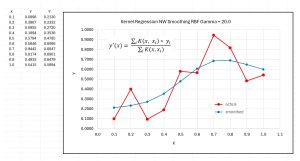 [Click on image for larger view.] Figure 2: Nadaraya-Watson Kernel Regression Used for Data Smoothing
In addition to prediction, NW kernel regression is often used for statistical data smoothing. The graph in Figure 2 shows NW kernel regression with 10 training data items, predicting the training data. A good value of RBF gamma generates a smooth interpolation of the data points.
About the Author
Dr. James McCaffrey directs the data science and research efforts at Quaetrix, a data analytics company located near Redmond, Washington. Before joining Quaetrix, James was a senior research engineer at Microsoft. James can be reached at [email protected].