The Data Science Lab
Linear Support Vector Regression Using C# with Particle Swarm Training
Dr. James McCaffrey from Microsoft Research presents a complete end-to-end demonstration of the linear support vector regression (linear SVR) technique, where the goal is to predict a single numeric value. A linear SVR model uses an unusual error/loss function and cannot be trained using standard techniques, and so particle swarm optimization training is used.
The goal of a machine learning regression problem is to predict a single numeric value. For example, you might want to predict a person's income based on their age, weight, current bank account balance, and so on. There are approximately a dozen common regression techniques. The most basic regression techniques are called linear because they assume the data falls along a straight line (or hyperplane) when graphed.
Linear techniques include ordinary linear regression, L1 (lasso) and L2 (ridge) regression, and linear support vector regression (linear SVR). This article presents a demo of linear SVR, implemented from scratch, using the C# language, with a particle swarm optimization training algorithm.
 [Click on image for larger view.] Figure 1: Linear Support Vector Regression Using Particle Swarm Training
A good way to see where this article is headed is to take a look at the screenshot in Figure 1. The demo program begins by loading synthetic training and test data into memory. The data looks like:
-0.1660,  0.4406, -0.9998, -0.3953, -0.7065,  0.4840
 0.0776, -0.1616,  0.3704, -0.5911,  0.7562,  0.1568
-0.9452,  0.3409, -0.1654,  0.1174, -0.7192,  0.8054
 0.9365, -0.3732,  0.3846,  0.7528,  0.7892,  0.1345
. . .
The first five values on each line are the x predictors. The last value on each line is the target y to predict. The demo creates a linear SVR model, evaluates the model accuracy on the training and test data, and then uses the model to predict the target y value for x = [-0.1660, 0.4406, -0.9998, -0.3953, -0.7065].
The first part of the demo output shows how a linear support vector regression model is created:
Creating SVR linear model
Done
Setting SVR parameters:
C = 1.00
epsilon = 0.10
Linear support vector regression requires two parameters. The C value controls how much outlier data items are penalized in the loss function. The epsilon value controls which training data items are outliers. The C and epsilon values are free parameters and must be determined by trial and error.
The next part of the demo output shows how particle swarm optimization training is performed:
Setting particle swarm training parameters:
numParticles = 100
maxIter = 1000

Starting PSO training
iteration =      0  loss = 414.7436  acc (0.15) = 0.0050
iteration =    200  loss =   0.1774  acc (0.15) = 0.6200
iteration =    400  loss =   0.1774  acc (0.15) = 0.6200
iteration =    600  loss =   0.1774  acc (0.15) = 0.6200
iteration =    800  loss =   0.1774  acc (0.15) = 0.6200
Done
Particle swarm optimization training is inspired by simulated social behavior such as the movement of birds in a flock. Each possible solution is encapsulated in a particle object as the particle's position. The numParticles parameter sets the number of possible solutions. The maxIter parameter controls how many times each particle/solution "moves" towards a better position.
Loss/error quickly decreases and prediction accuracy increases, which indicate training is working. A prediction is scored as correct if it's within 15% of the true target value.
After training, the demo displays the linear SVR model weights (one per predictor variable) and the single bias value, which define the model. The demo also displays the weights and bias values that were obtained by using the Python language scikit-learn library. The scikit linear SVR model values are very close to the ones generated by the demo program:
Coefficients/weights:
-0.2588  0.0299  -0.0520  0.0259  -0.1014
Bias/constant/intercept: 0.3729

Coeffs via scikit / libsvm:
-0.2588  0.0300  -0.0520  0.0259  -0.1014
Intercept: 0.3729
The demo concludes by evaluating the final linear SVR model and making a prediction:
Evaluating model
Accuracy train (within 0.15) = 0.6200
Accuracy test (within 0.15) = 0.6750

Predicting for x =
 -0.1660  0.4406 -0.9998 -0.3953 -0.7065
0.5424
The model accuracy isn't very good -- only 62.00% accuracy on the training data (124 out of 200 correct) and 67.50% accuracy on the test data (27 out of 40 correct). The model has poor prediction accuracy because the synthetic demo data was generated by a neural network with random weights and biases, and so the data isn't linear (which you wouldn't know in advance in a non-demo scenario).
This article assumes you have intermediate or better programming skill but doesn't assume you know anything about linear support vector regression or particle swarm optimization. The demo is implemented using C# but you should be able to refactor the demo code to another C-family language if you wish. All normal error checking has been removed to keep the main ideas as clear as possible.
The source code for the demo program is too long to be presented in its entirety in this article. The complete code and data are available in the accompanying file download, and they're also available
online.
The Demo Data
The demo data is synthetic. It was generated by a 5-10-1 neural network with random weights and bias values. The idea here is that the synthetic data does have an underlying, but complex, non-linear structure which can be predicted.
All of the predictor values are between -1.0 and +1.0. There are 200 training data items and 40 test items. When using linear support vector regression, technically, it's not necessary to normalize/scale your data. But normalizing usually leads to a better prediction model, especially if some raw predictor values are very large (such as employee income) and some values are small (such as employee age).
Linear support vector regression is most often used with data that has strictly numeric predictor variables. It is possible to use linear SVR with mixed categorical and numeric data, by using one-over-n-hot encoding on categorical data (such as a variable color with possible values red, blue, green), and equal interval encoding on data that has inherent ordering (such as a variable size with possible values small, medium, large).
Understanding Linear Support Vector Regression
For regular linear regression (not linear SVR), with five predictor variables, the prediction equation is y' = (w0 * x0) + (w1 * x1) + (w2 * x2) + (w3 * x3) + (w4 * x4) + b. The xi are the predictor values. The wi are the model weights, also called the coefficients. The b is the model bias, also called the constant or the intercept. Linear SVR works in the same way except that the values of the weights and bias are determined in a different way than standard linear regression.
For example, the demo trained SVR model weights are (-0.2588, 0.0299, -0.0520, 0.0259, -0.1014), and the bias is 0.3729. For an input x = (-0.1660, 0.4406, -0.9998, -0.3953, -0.7065), the predicted y is:
y' = (w0 * x0) + (w1 * x1) + (w2 * x2) +(w3 * x3) + (w4 * x4) + b
   = (-0.2588 * -0.1660) +
     ( 0.0299 *  0.4406) +
     (-0.0520 * -0.9998) +
     ( 0.0259 * -0.3953) +
     (-0.1014 * -0.7065) + 0.3747
   = 0.0430 + 0.0132 + 0.0520 + -0.0102 + 0.0716 + 0.3729
   = 0.5424
For regular linear regression, during training, all data items contribute to the error/loss equally via mean squared error. But for linear support vector regression, items with predicted y values that are close (within a small distance epsilon) to actual target y values do not directly contribute to the loss. Only items where the predicted y value is greater than epsilon more than the true target y value contribute to the loss. This is called epsilon-insensitive loss. This idea is shown in Figure 2.
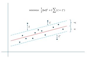 [Click on image for larger view.] Figure 2: Linear Support Vector Regression Epsilon-Insensitive Loss
The diagram in Figure 2 gives you a rough idea of support vector regression for a scenario where there is just one predictor variable x. Each dot is a training data item. The red line is the linear prediction equation created using epsilon-insensitive loss. The epsilon value (like a lower-case script 'e', often about 0.10 or so) creates a tube around the prediction equation. Data items that fall within the tube do not contribute to the loss value. Each data item that falls outside the tube generates a loss value usually denoted by Greek xi (looks like an upper-case script 'E').
The loss function is (1/2 * ||w||^2) + (C * sum(xi values)). The ||w||^2 is the squared vector norm of the weights (including bias). For example, if there are just three predictors, the linear prediction equation is y' = (w0 * x0) + (w1 * x1) + (w2 * x2) + b and ||w||^2 = w0^2 + w1^2 + w2^2 + b^2. The C is a free parameter, usually about 1.0 or 2.0. A larger value of C penalizes outlier data items more than a smaller value. The idea of minimizing the magnitudes of the weights is very subtle: it creates a "flatter" prediction equation, meaning the weight values are relatively in the same magnitude-range rather than wildly different. In machine learning terminology, this is called regularization.
Now here's where the difficulty of linear support vector regression arises. The loss function is not calculus-differentiable, which means that normal techniques for finding the values of the weights and bias don't work. In particular, you can't use the common stochastic gradient descent (SGD) optimization algorithm. This means you must either use extremely complex techniques like quadratic programming algorithms or use an algorithm like particle swarm optimization.
Understanding Particle Swarm Optimization
In high-level pseudo-code, particle swarm optimization is:
create a collection of possible random particles/solutions
    loop max_iter times
      compute new particle velocity based on
        1. current velocity
        2. best position/solution known to particle
        3. best position/solution known to all particles
      new position = curr position + new velocity
      keep track of best position/solution found so far
    end-loop
    return best position/solution found
The process is illustrated for two particles in Figure 3. For the demo problem with five predictor variables, a possible position/solution is a vector with six values: the five weights followed by the bias.
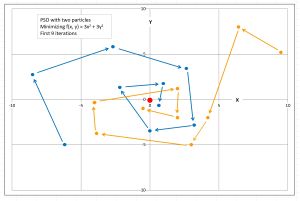 [Click on image for larger view.] Figure 3: Particle Swarm Optimization
Particle swarm optimization is a meta-heuristic rather than a specific algorithm, meaning there are many possible implementations. The movement of a particle is controlled by the particle's velocity which has three components. The first component is the current velocity. This is called inertia. The second component of velocity is the particle's best-known position. This is called the cognitive component. The third component is the best-known position found by any particle. This is called the social component.
Each of the three velocity components has an associated constant that determines its relative importance. Although these constants are free parameters, values of 0.729 (inertia weight), 1.49445 (cognitive weight), and 1.49445 (social weight) work well in practice. Each of the three velocity components are also modified by random values between 0.0 and 1.0 to inject a certain amount of randomness to prevent stalling out.
The Demo Program
I used Visual Studio 2022 (Community Free Edition) for the demo program. I created a new C# console application and checked the "Place solution and project in the same directory" option. I specified .NET version 8.0. I named the project SupportVectorRegressionLinearSwarm. I checked the "Do not use top-level statements" option to avoid the weird program entry point shortcut syntax.
The demo has no significant .NET dependencies and any relatively recent version of Visual Studio with .NET (Core) or the older .NET Framework will work fine. You can also use the Visual Studio Code program if you like.
After the template code loaded into the editor, I right-clicked on file Program.cs in the Solution Explorer window and renamed the file to the more descriptive SupportVectorRegressionSwarmProgram.cs. I allowed Visual Studio to automatically rename class Program.
The overall program structure is presented in Listing 1. All the control logic is in the Main() method in the Program class. The Program class also holds helper functions to load data from file into memory and display data. All of the linear support vector regression functionality is in a SupportVectorRegressorLinear class. The SupportVectorRegressorLinear class exposes a constructor and four methods: TrainSwarm(), Predict(), Accuracy(), and LossUsing().
Listing 1: Overall Program Structure
using System;
using System.IO;
using System.Collections.Generic;

namespace SupportVectorRegressionLinearSwarm
{
  internal class SupportVectorRegressionLinearSwarmProgram
  {
    static void Main(string[] args)
    {
      Console.WriteLine("Begin linear support vector " +
        "regression with particle swarm training demo ");

      // 1. load data
      // 2. create model
      // 3. train model
      // 4. show model weights and bias
      // 5. evaluate model
      // 6. use model to make a prediction

      Console.WriteLine("End demo ");
      Console.ReadLine();
    }

    static double[][] MatLoad(string fn, int[] usecols,
      char sep, string comment) { . . }

    static double[] MatToVec(double[][] mat) { . . }

    static void VecShow(double[] vec, int dec, int wid) { . . }
  }

  public class SupportVectorRegressor
  {
    // ------------------------------------------------------

    public class Particle
    {
      public double[] position; // soln = wts + bias
      public double loss;  // epsilon-insensitive
      public double[] velocity; // to determine next position

      public double[] bestPosition; // best seen
      public double bestLoss;

      public Particle(int solnLen)
      {
        this.position = new double[solnLen];
        this.velocity = new double[solnLen];
        this.bestPosition = new double[solnLen];
      }
    }

    // ------------------------------------------------------

    public double[] weights; // aka coefficients
    public double bias;  // aka constant, intercept
    private Random rnd;

    public SupportVectorRegressor(int seed) { . . }

    public double Predict(double[] x) { . . }

    public double Accuracy(double[][] dataX, double[] dataY,
      double pctClose) { . . }

    public void TrainSwarm(double[][] trainX, double[] trainY,
      double C, double epsilon,
      int numParticles, int maxIter) { . . }

    private double PredictUsing(double[] soln, double[] x) { . . }

    public double LossUsing(double[] soln,
      double[][] dataX, double[] dataY,
      double C, double eps) { . . }

    private double AccuracyUsing(double[] soln, double[][] dataX,
      double[] dataY, double pctClose) { . . }
   } // class SupportVectorRegressor
} // ns
The demo system encapsulates a possible solution and its associated epsilon-insensitive error/loss in a nested Particle class. The possible solution, five weights followed by a bias, are stored in a vector field named position.
Loading the Data into Memory
The demo program starts by loading the 200-item training data into memory:
string trainFile =
  "..\\..\\..\\Data\\synthetic_train_200.txt";
int[] colsX = new int[] { 0, 1, 2, 3, 4 };
double[][] trainX =
  MatLoad(trainFile, colsX, ',', "#");
double[] trainY =
  MatToVec(MatLoad(trainFile,
  new int { 5 }, ',', "#"));
The training X data is stored into an array-of-arrays style matrix of type double. The data is assumed to be in a directory named Data, which is located in the project root directory. The arguments to the MatLoad() function mean load columns 0, 1, 2, 3, 4 where the data is comma-delimited, and lines beginning with "#" are comments to be ignored. The training y data in column [5] is loaded into a matrix and then converted to a one-dimensional vector using the MatToVec() helper function.
The 40-item test data is loaded into memory using the same pattern that is used to load the training data:
string testFile =
  "..\\..\\..\\Data\\synthetic_test_40.txt";
double[][] testX =
  MatLoad(testFile, colsX, ',', "#");
double[] testY =
  MatToVec(MatLoad(testFile,
  new int[] { 5 }, ',', "#"));
The first three training items are displayed like so:
Console.WriteLine("First three train X: ");
for (int i = 0; i < 3; ++i)
  VecShow(trainX[i], 4, 8);
Console.WriteLine("First three train y: ");
for (int i = 0; i < 3; ++i)
  Console.WriteLine(trainY[i].ToString("F4").PadLeft(8));
In a non-demo scenario, you might want to display all the training data to make sure it was correctly loaded into memory.
Creating and Training the Model
The linear SVR model is created using these statements:
Console.WriteLine("Creating SVR linear model ");
SupportVectorRegressorLinear model =
  new SupportVectorRegressorLinear(seed: 0);
Console.WriteLine("Done ");
The model constructor accepts only a seed value for a Random object. Next, the demo prepares and performs training:
double C = 1.0;
double epsilon = 0.10;
int numParticles = 100;
int maxIter = 1000;
Console.WriteLine("Starting PSO training ");
model.TrainSwarm(trainX, trainY, C, epsilon, numParticles, maxIter);
Console.WriteLine("Done");
The C and epsilon values that are specific to the epsilon-insensitive error/loss calculation are declared separately and passed to the TrainSwarm() method. Linear support vector regression with particle swarm optimization training is sensitive to all four hyperparameters: C, epsilon, numParticles, and maxIter. These values must be determined by trial and error.
The demo program displays the five model weights and the bias:
Console.WriteLine("Coefficients/weights: ");
for (int i = 0; i < model.weights.Length; ++i)
  Console.Write(model.weights[i].ToString("F4") + "  ");
Console.WriteLine("Bias/constant/intercept: " +
  model.bias.ToString("F4"));
Because the this.weights and this.bias are public members of the SupportVectorRegressorLinear class, they can be accessed directly without the need for accessor properties. Very large weight values are not good and indicate that you should experiment with different hyperparameter values.
Evaluating and Using the Model
The demo program evaluates the trained model accuracy using these statements:
Console.WriteLine("Evaluating model ");
double accTrain = model.Accuracy(trainX, trainY, 0.15);
Console.WriteLine("Accuracy train (within 0.15) = " +
  accTrain.ToString("F4"));
double accTest = model.Accuracy(testX, testY, 0.15);
Console.WriteLine("Accuracy test (within 0.15) = " +
  accTest.ToString("F4"));
Accuracy is not a very granular metric. You can also use the public LossUsing() method to display the epsilon-insensitive loss, but this value isn't easy to interpret, other than smaller values are better. You could implement an error method that computes mean squared error, but linear SVR is not designed to minimize MSE.
The demo concludes by using the trained linear SVR model to predict the y value for the first training item, (-0.1660, 0.4406, -0.9998, -0.3953, -0.7065):
double[] x = trainX[0];
Console.WriteLine("Predicting for x = ");
VecShow(x, 4, 8);
double y = model.Predict(x);
Console.WriteLine(y.ToString("F4"));
The predicted y value, 0.5424, is not very close to the true target value of 0.4840. But, as mentioned previously, linear SVR is not well-suited for complex, non-linear data.
Wrapping Up
Linear support vector regression is now rarely used in practice. The idea was proposed in a 1998 research paper, but even that paper was mildly skeptical about how useful linear SVR could be. However, this didn't stop some researchers from investigating and promoting linear SVR in the late 1990s.
During training, linear support vector regression penalizes outlier data items more than non-outlier items via the C and epsilon constants, and keeps the magnitudes of the model weight and bias values small via the ||w||^2 term in the epsilon-insensitive error/loss function. However, L1 regression (also called lasso regression) and L2 regression (also called ridge regression), do the same things in a much simpler way. This was generally understood by about the year 2002 and linear SVR quickly lost favor with researchers and practitioners. However, you might run into linear SVR in a legacy system.