The Data Science Lab
Kernel Ridge Regression with Stochastic Gradient Descent Training Using C#
Dr. James McCaffrey presents a complete end-to-end demonstration of the kernel ridge regression technique to predict a single numeric value. The demo uses stochastic gradient descent, one of two possible training techniques. There is no single best machine learning regression technique. When kernel ridge regression prediction works, it is often highly accurate.
The goal of a machine learning regression problem is to predict a single numeric value. For example, you might want to predict a person's bank savings account balance based on their age, years of education, and so on.
There are approximately a dozen common regression techniques. Examples include linear regression, k-nearest neighbors regression, decision tree regression, and neural network regression. Each technique has pros and cons. A technique that often produces accurate predictions for complex data is called kernel ridge regression.
Kernel ridge regression uses a kernel function that computes a measure of similarity between two data items, and a ridge regularization technique to limit model overfitting. Model overfitting occurs when a model predicts well on the training data, but predicts poorly on new, previously unseen data. Ridge regularization is also known as L2 regularization.
This article presents a demo of kernel ridge regression, implemented from scratch, using the C# language. A good way to see where this article is headed is to take a look at the screenshot in Figure 1. The demo program begins by loading synthetic training and test data into memory. The data looks like:
-0.1660,  0.4406, -0.9998, -0.3953, -0.7065,  0.4840
 0.0776, -0.1616,  0.3704, -0.5911,  0.7562,  0.1568
-0.9452,  0.3409, -0.1654,  0.1174, -0.7192,  0.8054
 0.9365, -0.3732,  0.3846,  0.7528,  0.7892,  0.1345
. . .
The first five values on each line are the x predictors. The last value on each line is the target y variable to predict. There are 200 training items and 40 test items.
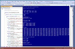 [Click on image for larger view.] Figure 1: Kernel Ridge Regression with SGD Training in Action
The demo creates and trains a kernel ridge regression model, evaluates the model accuracy on the training and test data, and then uses the model to predict the target y value for the first training item x = [-0.1660, 0.4406, -0.9998, -0.3953, -0.7065].
The first part of the demo output shows how a kernel ridge regression (KRR) model is created and trained:
Creating KRR object
Setting RBF gamma = 0.3
Setting alpha noise =  0.00001
Setting lrnRate = 0.0500
Setting maxEpochs = 2000

Training model
epoch =      0 MSE = 0.0181 acc = 0.1700
epoch =    400 MSE = 0.0001 acc = 0.9850
epoch =    800 MSE = 0.0000 acc = 0.9900
epoch =   1200 MSE = 0.0000 acc = 0.9850
epoch =   1600 MSE = 0.0000 acc = 0.9950
Done
Kernel ridge regression requires you to specify which kernel function to use. The demo uses the radial basis function (RBF) as the kernel function. The RBF kernel requires a value for a parameter called gamma. The alpha parameter controls the ridge regularization. The values of gamma and alpha must be determined by trial and error.
The demo program trains the KRR model using a technique called stochastic gradient descent (SGD). SGD training requires a value for a learning rate parameter, and a value for the maximum number of epochs to use. An epoch is one pass through all training data items. The values of the learning rate and the max epochs must be determined by trial and error.
The next part of the demo output shows the trained model weights:
Model weights:
-1.3278  -0.7593  -0.1208  -0.6889
 0.5953  -0.4384   0.6436   0.5068
. . .
-0.8158  -0.1501   0.0569   1.0963
A kernel ridge regression model has n weights where n is the number of training data items. Because the demo has 200 training items, the model has 200 weights. The weights are displayed so they can be inspected. Many extremely large positive or negative values, or mostly zero values, is not good and indicates possible model overfitting.
The demo concludes by evaluating the trained model and making a prediction:
Computing model accuracy (within 0.10)
Train acc = 0.9950
Test acc = 0.9500

Train MSE = 0.0000
Test MSE = 0.0002

Predicting for trainX[0]
Predicted y = 0.4948
The model accuracy is very good -- 99.5% accuracy on the training data (199 out of 200 correct) and 95.0% accuracy on the test data (38 out of 40 correct). A prediction is scored as correct if it's within 10% of the true target value.
The model mean squared error (MSE) values on the training and test data are very small, which is good. MSE is a more granular measure of model goodness than accuracy. MSE values are a good way to compare models when searching for model parameter values (gamma, alpha, learning rate, max epochs). The model's prediction for the first training item (-0.1660, 0.4406, -0.9998, -0.3953, -0.7065) is 0.4948 which is very close to the true target value of 0.4840.
This article assumes you have intermediate or better programming skill but doesn't assume you know anything about kernel ridge regression. The demo is implemented using C# but you should be able to refactor the demo code to another C-family language if you wish. All normal error checking has been removed to keep the main ideas as clear as possible.
The source code for the demo program is too long to be presented in its entirety in this article. The complete code and data are available in the accompanying file download, and they're also available online.
The Demo Data
The demo data is synthetic. It was generated by a 5-10-1 neural network with random weights and bias values. The idea here is that the synthetic data does have an underlying, but complex, non-linear structure which can be predicted.
All of the predictor values are between -1 and +1. When using kernel ridge regression, technically, it's not necessary to normalize/scale your data. But normalizing usually leads to a better prediction model, especially if some raw predictor values are very large (such as employee income) and some values are small (such as employee age).
The three most common techniques to normalize numeric data are min-max normalization, z-score normalization, and divide-by-constant normalization. When possible, I recommend divide-by-constant normalization. For example, if you have a predictor variable employee age, you could divide all age values by 100.
Kernel ridge regression is most often used with data that has strictly numeric predictor variables. It is possible to use the technique with categorical predictors. If a predictor variable has an inherent order, you can use equal-interval encoding. For example, a predictor variable height with possible values (short, medium, tall) could be encoded as short = 0.25, medium = 0.50, tall = 0.75.
For categorical predictor variables without inherent order, such as color with three possible values (red, blue, green), you can use one-over-n-hot encoding. For instance, red = (0.3333, 0, 0), blue = (0, 0.3333, 0), green = (0, 0, 0.3333). Unlike basic one-hot encoding, one-over-n-hot encoding takes into account the number of possible values of the predictor variable.
Understanding the RBF Kernel Function
In order to understand kernel ridge regression, you must understand the radial basis function (RBF) kernel function. The RBF kernel computes a measure of similarity between two vectors. There are two RBF versions. The RBF version used by the demo program is called the gamma version. The function is defined as:
rbf(v0, v1) = exp( -1 * gamma * ||v0 - v1||^2 )
Here, v0 and v1 are two vectors, exp() is the math e constant (2.71828...) raised to a power, ||v0 - v1||^2 is squared Euclidean distance, and gamma is an arbitrary constant. Gamma is sometimes called the inverse bandwidth, or just plain bandwidth, or width, or scale, or length. Sheesh.
Suppose v0 = (2.50, -3.25, 1.20) and v1 = (2.0, -3.0, 1.0) and gamma = 0.40. The trailing squared Euclidean distance term is the sum of the squared differences between vector elements:
||v0 - v1||^2 = (2.50 - 2)^2 + (-3.25 - (-3))^2 + (1.20 - 1)^2
              = (0.50)^2 + (-0.25)^2 + (0.20)^2
              = 0.2500 + 0.0625 + 0.0400
              = 0.3525

And then RBF(v0, v1) is:

rbf(v0, v1) = exp( -1 * gamma * ||v0 - v1||^2 )
            = exp( -1 * 0.40 * 0.3525 )
            = exp( -0.1410 )
            = 0.8685
If two vectors are the same, then rbf(v0, v1) = 1.0 (maximum similarity). As rbf(v0, v1) approaches but never quite reaches 0.0, it means the two vectors are less similar. RBF is symmetric so rbf(v0, v1) = rbf(v1, v0). Put another way, the RBF of two vectors is a value between 0 and 1 where larger values mean more similar.
Somewhat confusingly, there is a second definition for the RBF kernel function. It is:
rbf(v0, v1) = exp( -1 * ||v0 - v1||^2 / (2 * sigma^2) )
Here, instead of multiplying by an arbitrary constant gamma, you divide by 2 times the square of an arbitrary constant sigma. This version of RBF is sometimes called the sigma version.
Notice that gamma = 1 / (2 * sigma^2), and sigma = sqrt(1 / 2 * gamma). For the example vectors above, with gamma = 0.40, then sigma = sqrt(1 / 2*0.40) = sqrt(1.25) = 1.1180. If you use this value in the sigma version of the RBF definition, you will get the same 0.8685 result.
There are many different kernel functions. In machine learning scenarios, the RBF kernel function is the most common (at least, based on my experience), and is the one used by the demo program. Other, less commonly used kernel functions include the polynomial kernel, the sigmoid kernel, and the cosine kernel.
In math and research literature, a general kernel function is often written as K(x, x') to indicate any kernel function can be used. Sometimes kernel functions are defined so that they accept a just single vector, and you see K(x - x') to indicate you perform vector subtraction and then feed the result to the single-parameter kernel function.
To recap, kernel ridge regression uses a kernel function that compares two vectors. There are many different kernel functions. The most common is the radial basis function (RBF) kernel. The RBF kernel has two variations, the gamma version and the sigma version.
Kernel Ridge Regression Prediction
The kernel ridge regression prediction mechanism is best understood by looking at a concrete example. In words, to predict the y value for an input vector x, you compute the sum of the products of the model weights times the kernel function applied to x and each training item.
Suppose you have just three training data items, x0, x1, x2. A trained kernel ridge regression model will have three weights, w0, w1, w2. If the kernel function is the rbf() function, the predicted y for input x is:
y' = (w0 * rbf(x, x0)) + (w1 * rbf(x, x1)) + (w2 * rbf(x, x2))
For example, suppose the input x to predict is (2.0, 4.0, 1.0). And suppose that for some value of gamma, the RBF kernel function values are:
rbf(x, x0) = 0.80
rbf(x, x1) = 0.50
rbf(x, x2) = 0.90
And suppose the trained model weights are w0 = 0.60, w1 = 0.70, w2 = -0.20. The predicted y is:
y' = (w0 * rbf(x, x0)) + (w1 * rbf(x, x1)) + (w2 * rbf(x, x2))
   = (0.60 * 0.80) + (0.70 * 0.50) + (-0.20 * 0.90)
   = 0.48 + 0.35 + -0.18
   = 0.65
Many simple machine learning linear algorithms, such as linear regression, L1 (lasso) regression, and L2 (ridge) regression, require an additional weight, called the bias or intercept. For kernel ridge regression, the bias term is implicitly incorporated into the kernel function.
The demo Predict() method implementation is short and simple:
public double Predict(double[] x)
{
  int N = this.trainX.Length;
  double sum = 0.0;
  for (int i = 0; i < N; ++i) {
    double[] xx = this.trainX[i];
    double k = this.Rbf(x, xx);
    sum += this.wts[i] * k;
  }
  return sum;
}
OK. But where do the model weights come from?
Training a Kernel Ridge Regression Model
Training a kernel ridge regression model is the process of finding values for the n model weights (one per training item) so that predicted y values closely match the known correct target values in the training data.
There are two main ways to train a kernel ridge regression model. The first technique involves creating an n-by-n kernel matrix that compares all the training data items with each other. Then ridge regularization is applied by adding a small alpha constant to the diagonal elements of the kernel matrix. Then the matrix inverse of the kernel matrix is computed. The inverse of the kernel matrix is multiplied by the vector of training y values, which gives the model weights. This is called a closed-form solution for the model weights.
The second technique to train a kernel ridge regression model uses stochastic gradient descent (SGD). SGD is an iterative process that loops through the training data multiple times, adjusting the model weights slowly so that the model reduces its error between predicted y values and target y values. The demo program uses SGD training.
The matrix inverse training technique usually works well for small and medium size datasets. The matrix inverse technique has fewer training hyperparameters to deal with (no learning rate or maximum epochs) than the SGD technique. But the matrix inverse technique can't handle huge datasets, and matrix inverse computation is very complex and can fail even for small datasets.
The SGD training technique has more hyperparameters to tune than the matrix inverse technique. But the SGD technique is robust and can handle all sizes of datasets.
Expressed in high-level pseudo-code, the SGD training technique is:
    initialize weights to small random values
    loop max_epochs times
      shuffle order of training items
      loop each training item
        fetch input vector x and target y from train data
        compute predicted y using current weight values
        adjust associated weight so pred y is closer to target y
      end-loop (each training item)
      reduce all weights slightly using alpha
    end-loop
The order of the training items is shuffled on each pass through the data so that training doesn't oscillate, where the updates from one training item are repeatedly undone by updates to the next item.
The demo program does not use ridge/L2 regularization directly. Instead, weight decay is applied. The mathematical relationship between ridge regularization and weight decay is complicated, but both techniques deter weight model values from becoming large. Somewhat surprisingly, when using basic stochastic gradient descent, ridge/L2 regularization and weight decay are mathematically equivalent.
The key statements in the Train() method are:
double[] x = trainX[idx];
double predY = this.Predict(x);
double actualY = trainY[idx];
this.wts[idx] -= lrnRate * (predY - actualY);
The idx is the index of the current training item. If the predicted value is larger than the target value, the associated model weight is decreased by a percentage of the difference, lessened by multiplication by the learning rate value. Learning rate values are typically about 0.10 or 0.05. If the learning rate is too small, weights change slowly and training takes too long. If the learning rate is too large, weights change too much and good weight values get skipped.
The Demo Program
I used Visual Studio 2022 (Community Free Edition) for the demo program. I created a new C# console application and checked the "Place solution and project in the same directory" option. I specified .NET version 8.0. I named the project KernelRidgeRegressionSGD. I checked the "Do not use top-level statements" option to avoid the strange program entry point shortcut syntax.
The demo has no significant .NET dependencies and any relatively recent version of Visual Studio with .NET (Core) or the older .NET Framework will work fine. You can also use the Visual Studio Code program if you like.
After the template code loaded into the editor, I right-clicked on file Program.cs in the Solution Explorer window and renamed the file to the more descriptive KernelRidgeRegressionSGDProgram.cs. I allowed Visual Studio to automatically rename class Program.
The overall program structure is presented in Listing 1. All the control logic is in the Main() method in the Program class. All of the kernel ridge regression functionality is in a KRR class. The KRR class exposes a constructor and four methods: Train(), Predict(), Accuracy(), and MSE(). The private Shuffle() and Rbf() methods are used by the Train() and Predict() methods. The demo program has a utility class named Utils that contains static methods to load data from a text file into memory, and display data.
Listing 1: Overall Program Structure
using System;
using System.IO;
using System.Collections.Generic;

namespace KernelRidgeRegressionSGD
{
  internal class KernelRidgeRegressionSGDProgram
  {
    static void Main(string[] args)
    {
      Console.WriteLine("Begin C# kernel ridge " +
        "regression using SGD training ");

      // 1. load train and test data from file into memeory
      // 2. create KRR model
      // 3. train KRR model
      // 4. evaluate model accuracy
      // 5. use model to make a prediction

      Console.WriteLine("End KRR with SGD training demo ");
      Console.ReadLine();
    }
  }

  // ========================================================

  public class KRR
  {
    public double gamma;  // for RBF kernel
    public double alpha;  // regularization
    public double[][] trainX;  // need for prediction
    public double[] trainY;  // not needed this version
    public double[] wts;  // one per trainX item
    public Random rnd;

    public KRR(double gamma, double alpha, int seed = 1) { . .}

    public void Train(double[][] trainX, double[] trainY,
      double lrnRate, int maxEpochs) { . . }

    private void Shuffle(int[] indices) { . . }

    private double Rbf(double[] v1, double[] v2) { . . }

    public double Predict(double[] x) { . . }

    public double Accuracy(double[][] dataX,
      double[] dataY, double pctClose) { . . }

    public double MSE(double[][] dataX, double[] dataY) { . . }
  }

  // ========================================================

  public class Utils
  {
    public static double[][] MatLoad(string fn,
      int[] usecols, char sep, string comment) { . . }

    public static double[] MatToVec(double[][] mat) { . . }

    public static void MatShow(double[][] m, int dec,
      int wid) { . . }

    public static void VecShow(double[] vec, int dec,
      int wid) { . . }
  }

} // ns
The KRR class declares its six fields with public scope so that they can be accessed directly. Unlike some regression techniques, kernel ridge regression needs access to the X training predictor data because the Predict() method uses that data. The training target y values are not needed by the demo implementation, but they are stored anyway. The Random object is used by the Shuffle() method, which in turn is used by the Train() method, to shuffle the order of the training data during training.
Loading the Data into Memory
The demo program starts by loading the 200-item training data into memory:
string trainFile = "..\\..\\..\\Data\\synthetic_train_200.txt";
double[][] trainX = Utils.MatLoad(trainFile,
  new int[] { 0, 1, 2, 3, 4 }, ',', "#");
double[] trainY = Utils.MatToVec(Utils.MatLoad(trainFile,
  new int[] { 5 }, ',', "#"));
The training X data is stored into an array-of-arrays style matrix of type double. The data is assumed to be in a directory named Data, which is located in the project root directory. The arguments to the MatLoad() function mean load columns 0, 1, 2, 3, 4 where the data is comma-delimited, and lines beginning with "#" are comments to be ignored. The training y data in column [5] is loaded into a matrix and then converted to a one-dimensional vector using the MatToVec() helper function.
The 40-item test data is loaded into memory using the same pattern that was used to load the training data:
string testFile = "..\\..\\..\\Data\\synthetic_test_40.txt";
double[][] testX = Utils.MatLoad(testFile,
  new int[] { 0, 1, 2, 3, 4 }, ',', "#");
double[] testY = Utils.MatToVec(Utils.MatLoad(testFile,
  new int[] { 5 }, ',', "#"));
The first three training items are displayed with four decimals like so:
Console.WriteLine("First three X predictors: ");
for (int i = 0; i < 3; ++i)
  Utils.VecShow(trainX[i], 4, 9);
Console.WriteLine("\nFirst three target y: ");
for (int i = 0; i < 3; ++i)
  Console.WriteLine(trainY[i].ToString("F4").PadLeft(8));
In a non-demo scenario, you might want to display all the training data to make sure it was correctly loaded into memory.
Creating and Training the Model
The kernel ridge regression model is created like so:
double gamma = 0.3;    // RBF param
double alpha = 1.0e-5;  // regularization
Console.WriteLine("Setting RBF gamma = " + gamma.ToString("F1"));
Console.WriteLine("Setting alpha noise =  " + alpha.ToString("F5"));
KRR krr = new KRR(gamma, alpha);
As mentioned previously, good values for gamma and alpha must be determined by trial and error. You can do this manually or programmatically. The KRR constructor has a parameter named seed that is used to initialize the Random object that controls the shuffling of the order in which training data items are processed by the Train() method. The seed parameter has a default value of 1. The value of seed will affect the accuracy of the resulting model, but you shouldn't treat seed as a parameter to be tuned.
Next, the demo prepares the training parameters and calls the Train() method:
double lrnRate = 0.05;
int maxEpochs = 2000;
Console.WriteLine("Setting lrnRate = " + lrnRate.ToString("F4"));
Console.WriteLine("Setting maxEpochs = " + maxEpochs);
Console.WriteLine("Training model ");
krr.Train(trainX, trainY, lrnRate, maxEpochs);
Console.WriteLine("Done ");
Console.WriteLine("Model weights: ");
Utils.VecShow(krr.wts, 4, 9);
In a non-demo scenario, you can programmatically try different values for the training parameters using a grid search along the lines of:
double[] rates = new double[] { 0.001, 0.005, 0.010, 0.050 };
int[] epochs = new int[] { 50, 100, 500, 1000, 2000, 5000 };
foreach (double lrnRate in rates) {
  foreach (int maxEpoch in epochs) {
    KRR model = new KRR(0.3, 1.0e-5);
    model.Train(trainX, trainY, lrnRate, maxEpoch);
    // compute and display accuracy and error
  }
}
After training has completed, the demo program displays the model weights:
Console.WriteLine("\nModel weights: ");
Utils.VecShow(krr.wts, 4, 9);
Console.WriteLine("Model bias/intercept: " +
  model.bias.ToString("F4").PadLeft(8));
In a non-demo scenario, instead of visually examining the model weights for weirdnesses, you can programmatically analyze by computing the largest and smallest weights, number of weights with 0 values, and so on.
Evaluating and Using the Model
The demo program evaluates the trained model using these statements:
double trainAcc = krr.Accuracy(trainX, trainY, 0.10);
double testAcc = krr.Accuracy(testX, testY, 0.10);
Console.WriteLine("\nTrain acc = " + trainAcc.ToString("F4"));
Console.WriteLine("Test acc = " +  testAcc.ToString("F4"));

double trainMSE = krr.MSE(trainX, trainY);
double testMSE = krr.MSE(testX, testY);
Console.WriteLine("\nTrain MSE = " + trainMSE.ToString("F4"));
Console.WriteLine("Test MSE = " +  testMSE.ToString("F4"));
The Accuracy() method scores a prediction value as correct if it's within a specified percentage of the true target value. A reasonable closeness percentage to use will vary from problem to problem.
The MSE() method computes a more granular measure of model goodness than Accuracy(), but accuracy is easier to interpret and ultimately what you are usually most interested in. Most of the regression modules in the Python language scikit-learn library use the coefficient of determination, R-squared, as the primary evaluation metric. But in my opinion, mean squared error is preferable. You can easily implement a coefficient of determination method by using the MSE() method as a template.
The demo concludes by using the trained model to predict the y value for the first training item, (-0.1660, 0.4406, -0.9998, -0.3953, -0.7065):
double[] x = trainX[0];
Console.WriteLine("\nPredicting for trainX[0] ");
double y = krr.Predict(x);
Console.WriteLine("Predicted y = " + y.ToString("F4"));
The predicted y value, 0.4948, is very close to the true target value of 0.4840. This is a good result because the synthetic demo data was generated by a neural network, which has complex interactions between predictor variables.
In some scenarios, you might want to save the trained model weights so that the model can be used by other systems. The easiest way to do this is to implement a SaveWeights() method that writes a single line of comma-delimited model weight values to a specified text file. The weights can be loaded by implementing a LoadWeights() method.
Wrapping Up
This article presents a lot of information. To recap:
- Kernel ridge regression (KRR) is a machine learning technique to predict a numeric value.
- Kernel ridge regression requires a kernel function.
- A kernel function computes a measure of similarity between two training items.
- The most common kernel function is the radial basis function (RBF).
- There are two forms of the RBF function, the gamma and the sigma.
- There are two ways to train a KRR model, kernel matrix inverse and stochastic gradient descent (SGD).
- Both training techniques require an alpha constant for ridge (aka L2) regularization to deter model overfitting.
- The matrix inverse training technique often works well for small and medium size datasets, but it is complex and can fail.
- The SGD training technique can be used with any size dataset, but it requires a learning rate and a maximum epochs, which must be determined by trial and error.
- There is no single best machine learning regression technique. When kernel ridge regression prediction works, it is often highly accurate.