The Data Science Lab
Implementing k-Nearest Neighbors Regression Using JavaScript
Dr. James McCaffrey presents a complete end-to-end demonstration of k-nearest neighbors regression using JavaScript. There are many machine learning regression techniques, but k-nearest neighbors is especially simple to implement and the results are highly interpretable.
The goal of a machine learning regression problem is to predict a single numeric value. For example, you might want to predict an employee's salary based on age, current bank account balance, years of experience, and so on. There are roughly a dozen common regression techniques, including multiple linear regression, kernel ridge regression, tree-based regression (decision tree, AdaBoost, random forest, bagging, gradient boosting), neural network regression. Note that logistic regression, in spite of its name, is a binary classification algorithm, not a regression algorithm.
This article presents a demo of k-nearest neighbors (k-NN) regression using the JavaScript language. Compared to other regression techniques, k-NN regression is often (but not always) slightly less accurate, but k-NN regression is very simple to implement and customize, and k-NN regression results are highly interpretable.
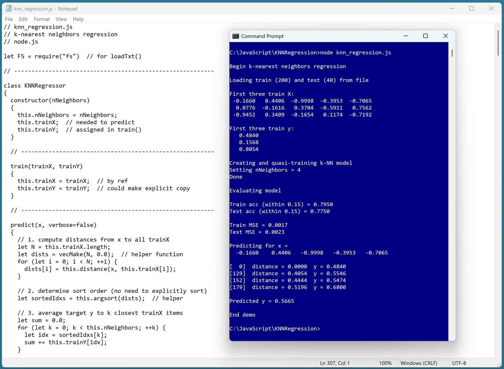 [Click on image for larger view.] Figure 1: The k-NN Regression Technique Using JavaScript in Action
A good way to see where this article is headed is to take a look at the screenshot in Figure 1. The demo program begins by loading synthetic training and test data into memory. dataset into memory. Behind the scenes, the data looks like:
-0.1660,  0.4406, -0.9998, -0.3953, -0.7065,  0.4840
 0.0776, -0.1616,  0.3704, -0.5911,  0.7562,  0.1568
-0.9452,  0.3409, -0.1654,  0.1174, -0.7192,  0.8054
 0.9365, -0.3732,  0.3846,  0.7528,  0.7892,  0.1345
. . .
The first five values on each line are the x predictors. The last value on each line is the target y variable to predict. The demo creates a k-NN regression model, evaluates the model accuracy on the training and test data, and then uses the model to predict the target y value for x = [-0.1660, 0.4406, -0.9998, -0.3953, -0.7065]. The key lines of the demo output are:
Creating and quasi-training k-NN model
Setting nNeighbors = 4

Evaluating model
Train acc (within 0.15) = 0.7950
Test acc (within 0.15) = 0.7750
Train MSE = 0.0017
Test MSE = 0.0023

Predicting for x =
-0.1660  0.4406 -0.9998 -0.3953 -0.7065
Predicted y = 0.5665
The k-NN regression technique is very simple. To make a prediction for some input vector x, you examine the training/reference data and find the k-closest items to x. The value of k is often set to a value between 3 and 7, and it must be determined by trial and error. The predicted y value is the average of the known y values of the close items in the training data.
This article assumes you have intermediate or better programming skill but doesn't assume you know anything about the k-NN regression algorithm. The demo is implemented using JavaScript running in a node.js environment, but you should be able to refactor the demo code to another C-family language if you wish. All normal error checking has been removed to keep the main ideas as clear as possible.
The source code for the demo program is a bit too long to be presented in its entirety in this article. The complete code and data are available in the accompanying file download, and they're also available online.
The Demo Data
The demo data is synthetic. It was generated by a 5-10-1 neural network with random weights and bias values. The idea here is that the synthetic data does have an underlying, but complex, structure which can be predicted.
All of the predictor values are between -1 and +1. When using k-NN regression, because nearest neighbors are computed using Euclidean distance, it's important to normalize the source data so that predictor variables with large magnitudes (for example, employee bank account balance) don't overwhelm variables with small magnitudes (for example, employee age). All the target values are between 0 and 1. There are 200 training/reference data items and 40 test items.
In practice, the k-NN regression technique is most often used with data that has strictly numeric predictor variables. It is possible to use k-NN regression with mixed categorical and numeric data.
Plain categorical data, such as a variable color with values "red," "blue," "green," can be one-over-n-hot encoded: red = (0.3333, 0, 0), blue = (0, 0.3333, 0), green = (0, 0, 0.3333). Categorical data with inherent ordering, such as a variable height with values "short," "medium," "tall," can be equal-interval encoded: short = 0.25, medium = 0.50, tall = 0.75. Binary data can be encoded using either technique for example, "male" = 0.0, "female" = 0.5 or "male" = 0.25, "female" = 0.75.
When using these encoding schemes, all encoded predictor magnitudes are between 0.0 and 1.0, and so numeric predictor data should be normalized too. The three most common normalization techniques are divide-by-constant, min-max normalization, and z-score normalization. When possible, I recommend using divide-by-constant normalization. For example, raw employee age values could be divided by 100.
Understanding k-NN Regression
The k-NN regression technique is perhaps best understood by looking at a concrete example. Suppose, as in the demo, you want to predict the y value for the first training/reference data item x = [-0.1660, 0.4406, -0.9998, -0.3953, -0.7065]. The algorithm scans through the 200 training/reference items and computes and saves the distance between x and each training item.
Next, the distances and their associated index values are sorted from smallest (nearest) distance to largest. For the demo data, the k = 4 nearest training data items to x are items [0], [129], [152], [179]:
[  0]  distance = 0.0000  y = 0.4840
[129]  distance = 0.4054  y = 0.5546
[152]  distance = 0.4444  y = 0.5474
[179]  distance = 0.5196  y = 0.6800
The predicted y value is the average of the y values of the nearest neighbors: y' = (0.4840 + 0.5546 + 0.5474 + 0.6800) / 4 = 2.2660 / 4 = 0.5665.
Because of the simple way in which k-NN regression works, it is highly interpretable. Any prediction can be clearly and unambiguously explained. In some scenarios, the high interpretability of k-NN regression trumps the better accuracy of difficult-to-interpret techniques such as AdaBoost regression and neural network regression.
The k-NN regression technique is somewhat different from most other regression techniques. The k-NN technique doesn't explicitly use training data to create a mathematical model (such as the linear regression technique or the neural network regression technique), after which the training data is no longer needed. Instead, in k-NN regression, the training data is, in effect, the model.
To make a prediction for an input vector x, it must be compared against all the training data to find the nearest neighbors. Because of this, training data for k-NN regression is sometime called reference data, and the method to train a k-NN regression model is sometimes named "quasi-training" or "fit" instead of "train."
One consequence of the data-is-the-model characteristic of k-NN regression is that if you want to save the model for later use or use by a different system, you must save the training data.
To compute closest neighbors, the demo implementation uses basic Euclidean distance. This is sometimes called Minkowsi distance with p = 2. There are other distance metrics, but they are rarely used.
The Demo Program
To code the demo, I used the old Notepad. I like the old Notepad. I'm not a fan of the current multiple-tabs Notepad. But you will probably want to use your regular text editor of choice.
I ran the demo program using the node.js runtime system. You can get node.js from nodejs.org/en/download. Any relatively recent version will work fine.
The overall program structure is presented in Listing 1. All the control logic is in the main() function. All the k-nearest neighbors regression functionality is in a KNNRegressor class. The KNNRegressor class exposes five methods: a constructor(), predict(), train(), accuracy(), and meanSqError(). Methods distance() and argsort() are helpers for the predict() method. The demo program implements six helper functions for the main() function: vecMake(), matMake(), vecShow, matShow(), matToVec(), loadTxt().
Listing 1: Overall Program Structure
// knn_regression.js
// k-nearest neighbors regression
// node.js

let FS = require("fs")  // for loadTxt()

// ----------------------------------------------------------

class KNNRegressor
{
  constructor(nNeighbors) { . . }
  train(trainX, trainY) { . . }
  predict(x, verbose=false) { . . }
  accuracy(dataX, dataY, pctClose) { . . }
  meanSqError(dataX, dataY) { . . }
  distance(v1, v2) { . . }
  argsort(vec) { . . }
}

// helper functions:

function vecMake(n, val) { . . }
function matMake(nRows, nCols, val) { . . }
function vecShow(vec, dec, wid, nl) { . . }
function matShow(M, dec, wid) { . . }
function matToVec(M) { . . }
function loadTxt(fn, delimit, usecols, comment) { . . }

// ----------------------------------------------------------

function main()
{
  console.log("Begin k-nearest neighbors regression ");

  // 1. load data from file into memory
  // 2. create and train k-NN regression model
  // 3. evaluate model
  // 4. use model

  console.log("End demo");
}

main();
The demo starts by loading the 200-item training data into memory:
let trainFile = ".\\Data\\synthetic_train_200.txt";
let trainX = loadTxt(trainFile, ",", [0,1,2,3,4], "#");
let trainY = loadTxt(trainFile, ",", [5], "#");
trainY = matToVec(trainY);
The training x data is stored into an array-of-arrays style matrix. The data is assumed to be in a directory named Data, which is located in the project root directory. The arguments to the loadTxt() function mean load columns 0, 1, 2, 3, 4 where the data is comma-delimited, and lines beginning with "#" are comments to be ignored. The training y data in column [5] is loaded into a matrix and then converted to a one-dimensional vector using the matToVec() helper function.
The 40-item test data is loaded into memory using the same pattern used for the training data:
let testFile = ".\\Data\\synthetic_test_40.txt";
let testX = loadTxt(testFile, ",", [0,1,2,3,4], "#");
let testY = loadTxt(testFile, ",", [5], "#");
testY = matToVec(testY);
The first three training items are displayed like so:
console.log("First three train X: ");
for (let i = 0; i < 3; ++i)
  vecShow(trainX[i], 4, 8, true);

console.log("First three train y: ");
for (let i = 0; i < 3; ++i)
  console.log(trainY[i].toFixed(4).toString().padStart(9, ' '));
In a non-demo scenario, you might want to display all the training data to make sure it was correctly loaded into memory.
If you are running k-NN regression inside a web page, you'll need to access training and test data in some other way. My blog post shows an example of a web page that uses HTML FileReader to fetch client-side data, and displays output in an HTML textarea zone. Another possibility is to fetch server-side data from a SQL database.
Creating and Training the k-NN Regression Model
The k-NN regression model is trained/fitted using these statements:
console.log("Creating and quasi-training k-NN model ");
let nNeighbors = 4;
console.log("Setting nNeighbors = " + nNeighbors.toString());
let model = new KNNRegressor(nNeighbors);
model.train(trainX, trainY);
console.log("Done ");
The number of nearest neighbors must be determined by trial and error. In most problem scenarios, you can do this manually, rather than programmatically examining different values.
The train() method doesn't do anything except store a reference copy of the training X and y data. If you customize the code presented in this demo so that the training data is modified, you might want to edit the train() method so that it saves an explicit value copy of the data instead of a reference copy.
Evaluating the k-NN Regression Model
The model accuracy evaluated using these statements:
console.log("Evaluating model ");
let trainAcc = model.accuracy(trainX, trainY, 0.15);
let testAcc = model.accuracy(testX, testY, 0.15);

console.log("Train acc (within 0.15) = " +
  trainAcc.toFixed(4).toString());
console.log("Test acc (within 0.15) = " +
  testAcc.toFixed(4).toString());
The accuracy() method scores a prediction as correct if it is within a specified percent of the true target value. The demo uses 0.15 as the percentage. A reasonable percentage threshold will vary from problem to problem.
The demo computes and displays the model mean squared error:
let trainMSE = model.meanSqError(trainX, trainY);
let testMSE = model.meanSqError(testX, testY);

console.log("Train MSE = " +
  trainMSE.toFixed(4).toString());
console.log("Test MSE = " +
  testMSE.toFixed(4).toString());
Mean squared error is a more granular metric than accuracy. In situations where the target y values have units, such as dollars for employee salary in dollars, you might want to use root mean squared error so that the metric is in dollars rather than squared-dollars.
The primary evaluation metric of the KNeighborsRegressor module of the Python language scikit-learn code library is the coefficient of determination, R2. In my opinion, mean squared error (or root mean squared error) is preferable in most situations. If you want to implement a coefficient of determination matrix, it's easy to do so by using the demo meanSqError() function as a template.
Using the k-NN Regression Model
The demo concludes by using the k-NN regression model to make a prediction:
let x = trainX[0];
console.log("Predicting for x = ");
vecShow(x, 4, 9, true);  // add newline

let predY = model.predict(x, true); // verbose
console.log("Predicted y = " + predY.toFixed(4).toString());
console.log("End demo");
The predict() method has a verbose parameter. When verbose is set to true, the predict() method() displays the indices of the closest training/reference data neighbors, and the distances from the item-to-predict and those neighbors:
Predicting for x =
-0.1660  0.4406  -0.9998  -0.3953  -0.7065

[  0]  distance = 0.0000  y = 0.4840
[129]  distance = 0.4054  y = 0.5546
[152]  distance = 0.4444  y = 0.5474
[179]  distance = 0.5196  y = 0.6800

Predicted y = 0.5665
An alternative design is to implement a predict() method without a verbose parameter, and a separate explain() method that displays closest indices and distances.
Wrapping Up
The k-NN regression system presented in this article is the simplest possible version. In the early days of machine learning, several variations of k-NN regression were explored, for example, weighting the predicted value by the distances to the nearest neighbors, or using the median of the y values of the closest neighbors. In most cases, the added complexity of these variations does not significantly improve k-NN regression and so the variations are not widely used today.