The Data Science Lab
ANOVA Using JavaScript
Analysis of variance (ANOVA) is a classical statistics technique that's used to infer if the unknown means (averages) of three or more groups are likely to all be equal or not, based on the variances of samples from the groups. For example, imagine that there are four high schools and you want to know if the average math abilities of students in the four schools are the same or not.
Suppose that it's too difficult and expensive to give all the students in the four schools a math test. So you randomly select 10 students from each school and give them the test. Some of the students fail to take the test so not all groups have the same size. You can use ANOVA to infer if the average math ability in all four schools is the same or not.
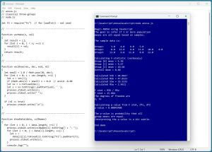 [Click on image for larger view.] Figure 1: ANOVA Using JavaScript in Action
A good way to see where this article is headed is to take a look at the screenshot of a demo program in Figure 1. The first part of the demo output is:
The sample data is:
Group1:     3.0    4.0    6.0    5.0
Group2:     8.0   12.0    9.0   11.0   10.0    8.0
Group3:    13.0    9.0   11.0    8.0   12.0

Group [0] mean = 4.50
Group [1] mean = 9.67
Group [2] mean = 10.60
Overall mean = 8.60
The demo program sets up three samples: (3, 4, 6, 5), (8, 12, 9, 11, 10, 8), and (13, 9, 11, 8, 12) from three unknown populations. The means of the three samples are 4.50, 9.67, and 10.60. The overall mean of the 15 sample values is 8.60. The means of the second and third sample groups look similar, but the mean of the first sample is quite a bit lower than the other two. You immediately suspect that the unknown population means are not all the same.
The next part of the demo output is:
Calculated SSb = 94.0667
Calculated MSb = 47.0333
Calculated SSw = 35.5333
Calculated MSw = 2.9611

F stat = MSb / MSw
F stat = 15.884
The degrees of freedom are 2, 12
The demo program computes intermediate SSb and SSw ("sum of squared") values and uses them to compute MSb and MSw ("mean squared") values. The computed F-statistic is MSb / MSw = 15.884.
Each set of sample data in an ANOVA problem has two df ("degrees of freedom") values. In general, df1 = number groups minus one, and df2 = total number of values minus number groups. So for the demo data, df1 = 3 - 1 = 2, and df2 = 15 - 3 = 12.
The last part of the demo output is:
Calculating p-value from F stat, df1, df2
p-value = 0.00042480

The p-value is probability that all
group means are equal.
Interpreting the p-value is a bit subtle.
The F-statistic and the two df values are used to compute a p-value ~= 0.0004. The p-value, very loosely, is the probability that all three source population means are the same based on the evidence computed from the variances of the three samples. Because the p-value is so small, you would conclude it's unlikely that the three source populations from which the samples were selected all have the same mean.
The demo program does not check three ANOVA assumptions: 1.) the source data populations are all Normal (Gaussian, bell-shaped) distributed, 2.) the variances of the source data populations are the same, 3.) the sample observations are independent of each other. In practice, checking ANOVA assumptions is often not practical.
This article assumes you have intermediate or better programming skill with the JavaScript language but doesn't assume you know anything about ANOVA. The demo code is a bit too long to present in its entirety in this article, but you can find the complete source code in the accompanying file download, and also online.
Computing the F-Statistic
Computing the F-statistic from samples of data is best explained by example. Suppose, as in the demo, there are three groups of samples from three populations:
Group 1: 3, 4, 6, 5
Group 2: 8, 12, 9, 11, 10, 8
Group 3: 13, 9, 11, 8, 12
The means of each sample group and the overall mean are:
Mean 1: (3 + 4 + 6 + 5) / 4 = 18 / 4 = 4.50
Mean 2: (8 + 12 + . . + 8) / 6 = 58 / 6 = 9.67
Mean 3: (13 + 9 + . . + 12) / 5 = 53 / 5 = 10.60
Overall: (3 + 4 + . . + 12) / 15 = 129 / 15 = 8.60
The SSb ("sum of squares between groups") is the weighted sum of squared differences between each group mean and the overall mean:
SSb = 4 * (4.50 - 8.60)^2 +
      6 * (9.67 - 8.60)^2 +
      5 * (10.60 - 8.60)^2
    = 94.07
The MSb ("mean sum of squares between groups") = SSb / (k - 1) where k is the number of groups. For the demo data:
MSb = SSb / (3 - 1)
    = 94.07 / (3 - 1)
    = 47.03
The SSw ("sum of squares within groups") is the sum of squared differences between each sample data point and its associated group mean. For the demo data:
SSw = (3 - 4.50)^2 + (4 - 4.50)^2 + . . + (12 - 10.60)^2
    = 35.53
The MSw ("mean sum of squares within groups") = SSw / (N - k) where N is the total number of sample data points and k is the number of groups:
MSw = 35.53 / (15 - 3)
    = 35.53 / 12
    = 2.96
The computed F-statistic is MSb divided by MSw:
F-stat = MSb / MSw
       = 47.03 / 2.96
       = 15.88
The larger the computed F-statistic is, the more likely it is that the population means are not all the same. Note that "not all the same" is not equivalent to "all different."
Computing the P-Value from the F-Statistic
The p-value is the area under the associated F-distribution, from the computed F-statistic value to positive infinity. The idea is best explained using a graph. See Figure 2.
There isn't just one F-distribution, there are many. There is a different F-distribution for each pair of df1 and df2 values. This is similar to the way that there is a different Normal (Gaussian, bell-shaped) distribution for each pair of (mean, standard deviation) values.
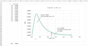 [Click on image for larger view.] Figure 2: Example of One F-Distribution
The graph in Figure 2 shows the F-distribution for df1 = 4 and df2 = 12 (not the df1 = 2, df2 = 12 of the demo data). Unlike the Gaussian distributions which all have a bell-shape, the shapes of different F-distributions look quite different from each other.
The total area under any F-distribution is exactly 1. The p-value is the area of the right-tail: the area under the curve from the F-statistic to positive infinity. In the graph, each rectangle has an area of 0.10. If you look closely, you can see that the area in the right-tail is about one rectangle, and in fact the exact p-value is 0.0982.
Computing the area under an F-distribution is difficult. There are several different approaches. The demo program uses the "regularized incomplete beta" function to compute a p-value. The regularized incomplete beta function is often written as Ix(a, b) or I(x; a, b). You can think of I(x; a, b) as an abstract black box math function that accepts an x value between 0.0 and 1.0 and positive a and b values.
Although the math is deep, computing a p-value from an F-statistic, df1 and df2 is simple:
x = df2 / (df2 + df1 * f-stat)
a = df2 / 2
b = df1 / 2
p-value = I(x, a, b)
This is easy if you have the I(x; a, b) function. But implementing the I(x; a, b) function is a very difficult problem in numerical programming. Briefly, I(x; a, b) can be computed using the log-beta function, and the log-beta function can be computed using the log-gamma function. The underlying beta and gamma functions are very complicated but you don't need to understand them fully in order to perform an ANOVA analysis.
The Demo Program
The demo program begins by setting up three groups of sample data:
function main()
{
  console.log("Begin ANOVA using JavaScript ");
  let data = vecMake(3, 0.0);
  data[0] = [3, 4, 6, 5];
  data[1] = [8, 12, 9, 11, 10, 8];
  data[2] = [13, 9, 11, 8, 12];
  let colNames = ["Group1", "Group2", "Group3"];

  console.log("The sample data is: ");
  showData(data, colNames);
. . .
The vecMake() function is a helper that creates a JavaScript array with three cells, all set to a 0.0 value. The array is expanded into an array-of-array styles matrix by assigning vectors to each cell. The showData() function is a helper to display the data in a nice format. Next, the demo data is used to find the computed F-statistic:
  console.log("Calculating F-statistic (verbosely)");
  let fstat = Fstat(data);
  console.log("F stat = " + fstat.toFixed(3).toString());
The program-defined Fstat() function computes group means, the overall mean, MSb and MSw as explained earlier.
The demo program concludes by computing and displaying the p-value from the degrees of freedom values and the f-statistic like so:
. . .
  let df1 = 3 - 1;  // k - 1
  let df2 = 15 - 3;  // N - k
  console.log("The degrees of freedom are ");
  console.log(df1.toString() + ", " + df2.toString());

  console.log("Calculating p-value from F stat, df1, df2 ");
  let pValue = FDist(fstat, df1, df2);

  process.stdout.write("p-value = ");
  console.log(pValue.toFixed(8).toString());
    console.log("End demo");
}
main();
The demo program hard-codes the df1 and df2 values. An alternative approach is to compute df1 and df2 programmatically from the sample data.
The FDist() Function
The key to the demo is the FDist() function that computes the p-value. It is defined as:
function FDist(fstat, df1, df2)
{
  // right tail of F-dist past fstat
  let x = df2 / (df2 + df1 * fstat);
  let a = df2 / 2;
  let b = df1 / 2;
  return regIncBeta(x, a, b);
}
The FDist() function is deceptively simple-looking because all of the difficult work is done by the regIncBeta() function. The regIncBeta() function is a wrapper over a regIncompleteBeta() function which calls helper functions logBeta() and contFraction(). The logBeta() function calls a logGamma() helper function. The logGamma() uses an interesting algorithm called the Lanczos approximation with g=5 and n=7.
Interpreting the Result
If all the (unknown) population means are the same, then when you sample from them, you'd expect the individual sample means and the overall mean to be about the same, subject to the randomness in sampling. This is called the mathematical null hypothesis. The computed p-value is probability that you'd see the sample means if in fact the population means are all the same. In other words, a small p-value means that it's unlikely that the unknown population means are all the same. A large p-value means it's quite possible that you'd see the sample data if all the population means are the same.
Put another way, a small p-value, such as p = 0.015 means, "If all the unknown population means are the same, and the two ANOVA assumptions that the unknown population data items are Gaussian distributed and have equal variances are true, then the probability that the sample means are as different as observed, is 0.015." Because this is a mouthful, it's common to loosely summarize by saying, "The probability that the population means are all the same is 0.015 and so the population means are likely not all the same."
If a p-value is not small, you can't conclude that, "the population means are all the same." It's better to say, "There's not enough statistical evidence to suggest that the population means are not all the same."
The point of all of this is that the results of an ANOVA analysis merely suggest whether all unknown population means are the same or not. An ANOVA analysis can never definitively prove anything about the population means.
Wrapping Up
One significant weakness of ANOVA is that it's often impossible to test the assumptions that the data sources are Gaussian distributed and have equal variances. This is another reason why ANOVA conclusions should be conservative.
An ANOVA analysis is intended for scenarios with three or more populations/groups. A closely related classical statistics technique is called the Student's t-test. The t-test is used to infer if the unknown means of exactly two populations are the same or not. It is possible to use ANOVA for just two groups, but the t-test is a more common approach. Mathematically, ANOVA with two groups is exactly equivalent to the t-test.
About the Author
Dr. James McCaffrey directs the data science and research efforts at Quaetrix, a data analytics company located near Redmond, Washington. Before joining Quaetrix, James was a senior research engineer at Microsoft. James can be reached at [email protected].