The Data Science Lab
Decision Tree Regression from Scratch with Pointers Using C#
Dr. James McCaffrey presents a complete end-to-end demonstration of decision tree regression from scratch using the C# language. The goal of decision tree regression is to predict a single numeric value. The demo implementation uses pointers (references) for efficiency but does not use any recursion for better maintainability and customization.
Decision tree regression is a machine learning technique that encapsulates a set of if-then rules in a tree data structure to predict a single numeric value. For example, a decision tree regression model prediction might be, "If employee age is greater than 43.0 and age is less than or equal to 51.5 and years-experience is less than or equal to 20.0 and height is greater than 58.0 then bank account balance is $845.41."
There are many ways to implement a decision tree regression system. Three major design decisions are 1.) use pointers/references for tree nodes, or use list storage, 2.) use recursion to construct the tree, or use a non-recursive stack, 3.) use mean squared error minimization for the node split function, or use variance reduction maximization.
This article presents decision tree regression, implemented from scratch with C#, using pointers/references for tree nodes, no recursion when building the tree, and using mean squared error minimaztion for the node split function.
A single decision tree can be used by iteself for regression problems. But a more common approach is to use a collection of decision trees for ensemble techniques: bagging tree regression, random forest regression, adaptive boosting regression, and gradient boosting regression. A decision tree regression system that uses pointers/references for tree nodes is well-suited for ensemble techniques.
A good way to see where this article is headed is to take a look at the screenshot in Figure 1 and the diagram in Figure 2. The demo program begins by loading synthetic training and test data into memory. The data looks like:
-0.1660,  0.4406, -0.9998, -0.3953, -0.7065,  0.4840
 0.0776, -0.1616,  0.3704, -0.5911,  0.7562,  0.1568
-0.9452,  0.3409, -0.1654,  0.1174, -0.7192,  0.8054
 0.9365, -0.3732,  0.3846,  0.7528,  0.7892,  0.1345
. . .
The first five values on each line are the x predictors. The last value on each line is the target y variable to predict. The demo creates a decision tree model, evaluates the model accuracy on the training and test data, and then uses the model to predict the target y value for x = [-0.1660, 0.4406, -0.9998, -0.3953, -0.7065].
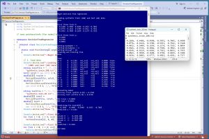 [Click on image for larger view.] Figure 1: Decision Tree Regression in Action on Synthetic Data.
The first part of the demo output shows how a decision tree is created:
Loading synthetic train (200) and test (40) data
Done

Setting maxDepth = 3
Setting minSamples = 2
Setting minLeaf = 18
Creating and training tree
Done
A decision tree regression system has three parameters that control the size and shape of the tree: maxDepth, minSaples, minLeaf. Briefly, maxDepth sets a maximum number of levels, and minSamples and minLeaf set node splitting granularity. For the demo, maxDepth is set to an artificially small value (3) and minLeaf is set to an artificially large value (18) to create a small tree that can be easily visualized.
The next part of the demo output displays the trained decision tree:
ID 0      0  -0.2102   not_null   not_null   0.0000  False
ID 1      4   0.1431   not_null   not_null   0.0000  False
ID 2      0   0.3915   not_null   not_null   0.0000  False
ID 3      0  -0.6553   not_null   not_null   0.0000  False
ID 4     -1   0.0000   null       null       0.4123   True
ID 5      4  -0.2987   not_null   not_null   0.0000  False
ID 6      2   0.3777   not_null   not_null   0.0000  False
ID 7     -1   0.0000   null       null       0.6952   True
ID 8     -1   0.0000   null       null       0.5598   True
ID 11    -1   0.0000   null       null       0.4101   True
ID 12    -1   0.0000   null       null       0.2613   True
ID 13    -1   0.0000   null       null       0.1882   True
ID 14    -1   0.0000   null       null       0.1381   True
The fields are node ID, index of split column (or -1 if the node cannot be split), split threshold (or 0.0000 if the node cannot be split), left child pointer/reference, right child pointer/reference, predicted y value (or 0.0000 if the node is not a predicting leaf node), and a Boolean indicating if the node is a leaf node (True) or not (False for split node). The tree is shown as a diagram in Figure 2.
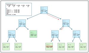 [Click on image for larger view.] Figure 2: Visual Representation of the Demo Decision Tree.
The next part of the demo output shows the tree model evaluation:
Evaluating model
Accuracy train (within 0.10) = 0.3750
Accuracy test (within 0.10) = 0.4750
MSE train = 0.0048
MSE test = 0.0054
The accuracy on the training data is very poor -- just 37.50% (75 correct out of 200). A prediction is scored as correct if it's withing 10% of the true target y value. The accuracy and MSE (mean squared error) are weak because maxDepth is too small and minLeaf is too large (to keep the tree small enough for easy visualization).
The last part of the demo output shows an example prediction:
Predicting for trainX[0] =
  -0.1660   0.4406  -0.9998  -0.3953  -0.7065
Predicted y = 0.4101

IF
column 0  >   -0.2102 AND
column 0  <=   0.3915 AND
column 4  <=  -0.2987 AND
THEN
predicted = 0.4101
One advantage of decision tree regression compared to other techniques, such as kernel ridge regression and neural network regression, is that decision trees are somewhat more interpretable. If you examine the diagram in Figure 2, and follow the red dashed arrows, you can see exactly how the predicted y value is computed.
This article assumes you have intermediate or better programming skill but doesn't assume you know anything about decision tree regression. The demo is implemented using C# but you should be able to refactor the demo code to another C-family language if you wish. All normal error checking has been removed to keep the main ideas as clear as possible.
The source code for the demo program is a too long to be presented in its entirety in this article. The complete code and data are available in the accompanying file download, and they're also available online.
The Demo Data
The demo data is synthetic. It was generated by a 5-10-1 neural network with random weights and bias values. The idea here is that the synthetic data does have an underlying, but complex, structure which can be predicted.
All of the predictor values are between -1 and +1. There are 200 training data items and 40 test items. When using decision tree regression, it's not necessary to normalize the training data predictor values because no distance between data items is computed. However, normalizing the predictors doesn't hurt and it's useful just in case you want to send the data to other regression algorithms that require normalization, for example, nearest neighbors regression and kernel ridge regression.
In practice, decision tree regression is most often used with data that has strictly numeric predictor variables. But it is possible to use decision regression with categorical data. For ordinal categorical data that has inherent ordering, you can use standard zero-based or one-based ordinal encoding. For example, for a predictor variable height with possible values (short, medium, tall), you could set short = 0, medium = 1, tall = 2.
For binary data, you can use zero-one encoding. For example, for a predictor variable sex, you could set male = 0, female = 1, or vice versa.
For nominal categorical data without inherent order, in theory, decision tree regression isn't applicable. But in practice, standard zero-based or one-based ordinal encoding often works well. For example, suppose you have a predictor variable race with possible values (Asian, Black, Hispanic, Mixed, White). You could set Asian = 0, Black = 1, Hispanic = 2, Mixed = 3, White = 4. One node of the decision tree might be, "If column [7] <= 2 Then go left." This would group Asian, Black, Hispanic together, and Mixed, White together.
The downside of ordinal encoding nominal categorical data is that the resulting tree has a significant dependency on the order in which you encode the data. The upside is that if the tree is deep enough, the technique often works well.
Understanding Decision Tree Regression - Splitting
The tree splitting part of constructing a decision tree regression system is perhaps best understood by looking at a concrete example. The root node of the demo decision tree is associated with all 200 rows of the training data. The splitting process selects some of the 200 rows to be assigned to the left child node, and the remaining rows to be assigned to the right child node.
For simplicity, suppose that instead of the demo training data with 200 rows and 5 columns of predictors, a tree node is associated with just 5 rows of data with 3 columns of predictors:
     X                    y
[0] 0.99  0.22  0.77     3.0
[1] 0.55  0.44  0.00     9.0
[2] 0.88  0.66  0.88     7.0
[3] 0.11  0.33  0.22     1.0
[4] 0.55  0.88  0.33     5.0
     [0]   [1]   [2]
The split algorithm wants to select some of the rows to go to the left child and the remaining rows to go to the right child. The idea is to select the two sets of rows in a way so that their associated y values are close together. You can do this by minimizing the mean squared error of the split, or maximizing the variance reduction of the split. The two techniques produce an identical split of rows but are implemented differently. The demo uses mean squared error minimization, mostly because it's a bit easier to implement than explicit variance reduction. There are other splitting algorithms, such as mean absolute deviation minimization, but they are generally used only in special scenarios.
The splitting algorithm examines every possible x value in every column. For each possible candidate split value (also called the threshold), the MSE of the resulting split is computed. For example, for x = 0.33 in column [1], the rows where the values in column [1] are less than or equal to 0.33 are rows [3] and [0] with associated y values (1.0, 3.0). The other rows are [1], [2], [4] with associated y values (9.0, 7.0, 5.0).
For this proposed split, the MSE of y values (1.0, 3.0) is the variance of the values. The mean of (1.0, 3.0) = (1.0 + 3.0) / 2 = 2.0 and the variance is ((3.0 - 2.0)^2 + (1.0 - 2.0)^2) / 2 = 1.00.
The mean of y values (9.0, 7.0, 5.0) = (9.0 + 7.0 + 5.0) / 3 = 7.0 and the variance is ((9.0 - 7.0)^2 + (7.0 -7.0)^2 + (5.0 - 7.0)^2) / 3 = 2.67.
Because the proposed split has different numbers of rows (two rows for the left child and three rows for the right child), the weighted MSE of the proposed split is computed: ((2 * 1.00) + (3 * 2.67)) / 5 = 2.00.
This process is repeated for every x value in every column. The x value and its column that generate the smallest weighted MSE define the split. In practice it's common to keep track of which values in a given column have already been checked, to avoid unnecessary work. The predicted y value for a leaf node (no further splits) is just the average of the y values associated with the node.
A common source of minor confusion is that the term "mean squared error" has two different meanings in machine learning. In most scenarios, mean squared error is the average of the squared differences between predicted y values and correct target y values, and it is used to evaluate the predictive accuracy of a trained model. But in decision tree splitting contexts, mean squared error is the exact same as statisical variance. The idea is that in a decision tree, the predicted values are the y values of a split and the virtual correct target y values are all identical, the mean of the y values.
Implementing the Split Function
When implementing a split function, the minSamples parameter specifies the minimum number of rows associated with a node necessary before a split is to be considered. In practice this is usually set to 2 which leads to many splits and a more granular tree.
The minLeaf parameter specifies the minimum number of rows required after a split is performed. In practice this is usually set to 1 which allows leaf nodes with a single associated y value, but prohibits any empty leaf nodes with no associated y values.
A common practice is to randomly shuffle the order in which columns are examined. The idea here is that without shuffling, the first predictor columns have priority over later columns in cases where there are multiple split values that produce the same minimum mean squared error. Shuffling the order of columns prevents a bias towards early columns, but introduces a small amount of randomness into a decision tree regression system.
The demo DecisionTreeRegressor class constructor has a parameter numSplitCols that specifies how many of the columns of the X data should be examined when looking for a split value and split column. In almost all scenarios, you want to examine all columns. An exception is when a collection of decision trees is used for a random forest regression system where there are many predictor variables. The constructor has a default value of -1 for numSplitCols which is a special value that means to use all columns.
Understanding Decision Tree Regression - Building
There are two main approaches for building a regression decision tree: recursion or stack. The most common in online examples is to use recursion. I suspect this is mostly because building a decision tree using recursion is elegant and fancy. However, many of the production teams I have worked with have a formal ban on the use of any kind of recursion in production code. Recursive code is tricky to implement, tricky to debug, tricky to profile, and tricky to modify.
The demo does not use recursion to build the tree. Instead, the demo uses a stack data structure. In high-level pseudo-code:
    create empty stack
    push (root, currX, currY, depth)
    while stack not empty
      pop (currNode, currX, currY, currDepth)
      if at maxDepth or not enough data then
        node is a leaf, compute predicted = average of currY
      end-if
      compute split value and split column of currX, currY
      if unable to split then
        node is a leaf, compute predicted = average of currY
      end-if
      compute leftX, leftY, rightX, rightY
      create and push (leftNode, leftX, leftY, currDepth+1)
      create and push (rightNode, rightX, rightY, currDepth+1)
    end-while
The build-tree algorithm is short but somewhat tricky. The stack holds a tree node and its associated X and y data, and the current depth of the tree. An alternative design is to explicitly store associated X and y data in each node. The current depth of the tree is maintained so that the algorithm knows when maxDepth has been reached.
The Demo Program
I used Visual Studio 2022 (Community Free Edition) for the demo program. I created a new C# console application and checked the "Place solution and project in the same directory" option. I specified .NET version 8.0. I named the project DecisionTreeRegression. I checked the "Do not use top-level statements" option to avoid the program entry point shortcut syntax.
The demo has no significant .NET dependencies and any relatively recent version of Visual Studio with .NET (Core) or the older .NET Framework will work fine. You can also use the Visual Studio Code program if you wish.
After the template code loaded into the editor, I right-clicked on file Program.cs in the Solution Explorer window and renamed the file to the slightly more descriptive DecisionTreeProgram.cs. I allowed Visual Studio to automatically rename class Program.
The overall program structure is presented in
Listing 1. All the control logic is in the Main() method in the Program class. The Program class also holds helper functions to load data from file into memory and display data.
All of the decision tree regression functionality is in a DecisionTreeRegressor class, which contains a nested Node container class, and a nested StackInfo container class. The DecisionTreeRegressor class exposes a constructor and six methods: Train(), Predict(), Explain(), Accuracy(), MSE(), and Display().
Listing 1: Overall Program Structure
using System;
using System.Collections.Generic;
using System.IO;

namespace DecisionTreeRegression
{
  internal class DecisionTreeProgram
  {
    static void Main(string[] args)
    {
      Console.WriteLine("Begin decision tree regression ");

      // 1. load data
      // 2. create and train/build tree
      // 3. evaluate model
      // 4. use model

      Console.WriteLine("End demo ");
      Console.ReadLine();

    } // Main()

    // helpers for Main()

    static double[][] MatLoad(string fn, int[] usecols,
      char sep, string comment) { . . }

    static double[] MatToVec(double[][] mat) { . . }

    static void VecShow(double[] vec, int dec, int wid) { . . }
  }

  public class DecisionTreeRegressor
  {
    public int maxDepth;
    public int minSamples;  // aka min_samples_split
    public int minLeaf;  // min number of values in a leaf
    public int numSplitCols; // mostly for random forest
    public Node root;
    public Random rnd;  // order in which cols are searched

    // ------------------------------------------------------

    public class Node // nested class
    {
      public int id;
      public int colIdx;  // aka featureIdx
      public double thresh;
      public Node left;
      public Node right;
      public double value;
      public bool isLeaf;

      public Node(int id, int colIdx, double thresh,
        Node left, Node right, double value, bool isLeaf) { . . }

      public void Show() { . . }
    }

    // --------------------------------------------

    public class StackInfo  // nested class to build tree
    {
      public Node node;
      public double[][] dataX;
      public double[] dataY;
      public int depth;

      public StackInfo(Node n, double[][] X, double[] y,
        int d) { . . }
    }

    // --------------------------------------------

    public DecisionTreeRegressor(int maxDepth = 2,
      int minSamples = 2, int minLeaf = 1,
      int numSplitCols = -1, int seed = 0) { . . } // ctor

    private double[] BestSplit(double[][] dataX,
      double[] dataY) { . . }

    private static void Shuffle(int[] indices, Random rnd) { . . }
    private static double Mean(List<double> values) { . . }
    private static double MSE(List<double> values) { . . }

    private Node MakeTree(double[][] dataX, double[] dataY,
      int depth = 0) { . . }
    private double[][] ExtractRows(double[][] source,
      List<int> rowIdxs) { . . }
    private double[] ExtractVals(double[] source,
      List<int> idxs) { . . }

    public void Train(double[][] trainX, double[] trainY) { . . }

    public double Predict(double[] x) { . . }
    public void Explain(double[] x) { . . }

    public double Accuracy(double[][] dataX, double[] dataY,
      double pctClose) { . . }
    public double MSE(double[][] dataX, double[] dataY) { . . }

    public void Display() { . . }

  } // class DecisionTreeRegressor
} // ns
The demo starts by loading the 200-item training data into memory:
string trainFile = "..\\..\\..\\Data\\synthetic_train_200.txt";
int[] colsX = new int[] { 0, 1, 2, 3, 4 };
double[][] trainX = MatLoad(trainFile, colsX, ',', "#");
double[] trainY = MatToVec(MatLoad(trainFile,
  new int[] { 5 }, ',', "#"));
The training X data is stored into an array-of-arrays style matrix of type double. The data is assumed to be in a directory named Data, which is located in the project root directory. The arguments to the MatLoad() function mean load columns 0, 1, 2, 3, 4 where the data is comma-delimited, and lines beginning with "#" are comments to be ignored. The training y data in column [5] is loaded into a matrix and then converted to a one-dimensional vector using the MatToVec() helper function.
The 40-item test data is loaded into memory using the same pattern that was used to load the training data:
string testFile = "..\\..\\..\\Data\\synthetic_test_40.txt";
double[][] testX = MatLoad(testFile, colsX, ',', "#");
double[] testY = MatToVec(MatLoad(testFile,
  new int[] { 5 }, ',', "#"));
Next, the first three training items are displayed like so:
Console.WriteLine("First three train X: ");
for (int i = 0; i < 3; ++i)
  VecShow(trainX[i], 4, 8);
Console.WriteLine("First three train y: ");
for (int i = 0; i < 3; ++i)
  Console.WriteLine(trainY[i].ToString("F4").PadLeft(8));
In a non-demo scenario, you might want to display all the training data to make sure it was correctly loaded into memory. The decision tree regression model is trained/fit/constructed using these statements:
int maxDepth = 3;
int minSamples = 2;
int minLeaf = 18;
// display the three parameters
Console.WriteLine("Creating and training tree ");
DecisionTreeRegressor tree =
  new DecisionTreeRegressor(maxDepth, minSamples,
    minLeaf, numSplitCols: -1, seed:0);
tree.Train(trainX, trainY);
Console.WriteLine("Done ");
Console.WriteLine("Tree: ");
tree.Display();
If maxDepth is set to 0, the tree has just a single (root) node and the predicted y value for any input is the average of the training y data. If maxDepth is set to 1, the tree has at most three nodes: root node, left child, right child. If maxDepth is set to 2, the tree has at most seven nodes. In general, if maxDepth is set to n, the tree has at most 2^(n+1)-1 nodes.
Decision trees are often sensitive to pathological data, and it's usually a good idea to display a trained tree to look for various weirdnesses. Next, the demo evaluates model accuracy:
double accTrain = dtr.Accuracy(trainX, trainY, 0.10);
Console.WriteLine("Accuracy train (within 0.10) = " +
  accTrain.ToString("F4"));
double accTest = dtr.Accuracy(testX, testY, 0.10);
Console.WriteLine("Accuracy test (within 0.10) = " +
  accTest.ToString("F4"));
The Accuracy() method scores a prediction as correct if the predicted y value is within 10% of the true target y value. The 10% is arbitrary and a reasonable closeness percentage will vary from problem to problem.
The demo computes model mean squared error using these statements:
double mseTrain = tree.MSE(trainX, trainY);
Console.WriteLine("MSE train = " +  mseTrain.ToString("F4"));
double mseTest = tree.MSE(testX, testY);
Console.WriteLine("MSE test = " + mseTest.ToString("F4"));
Recall that in decision tree terminology, MSE can refer to variance when computing split rows. This code is standard MSE which is a measure of how well the model predicts. The demo concludes by using the trained decision tree to make a prediction in two ways:
double[] x = trainX[0];
Console.WriteLine("Predicting for x = ");
VecShow(x, 4, 9);
double predY = tree.Predict(x);
Console.WriteLine("y = " + predY.ToString("F4"));
tree.Explain(x);
The Predict() method spits out the predicted y value without any explanation. The Explain() method is essentially a verbose predict function.
Wrapping Up
Implementing decision tree regression from scratch requires a bit of effort, but it allows you to easily integrate a prediction model with other systems. A from-scratch implementation also allows you to easily modify the system. For example, you can comment-out the code statements that shuffle the order in which columns are processed in the split function, so that your decision tree is completely deterministic, and you can add only error-checking that's relevant for your scenario.
The biggest disadvantage of a simple decision tree regression system is that a single tree usually overfits the training data. In overfitting, the trained model predicts well on the training data, but predicts poorly on new, previously unseen data. Because of the overfitting problem, decision trees are rarely used by themselves. Instead, multiple tress are combined into an ensemble model such as bagging tree regression, random forest regression, adaptive boosting regression, or gradient boosting regression.
The demo implementation uses pointers/references to connect the nodes in the decision tree. This approach is efficient but because references are memory addresses, they vanish after the program finishes, and so you can't directly save a trained model. This usually isn't a problem. In situations where a tree must be saved, you can serialize the tree nodes into a list data structure where the memory pointers/references are replaced by integer index values into the list.