The Data Science Lab
Quadratic Regression with Pseudo-Inverse Training Using C#
The goal of a machine learning regression problem is to predict a single numeric value. For example, you might want to predict a person's credit rating based on age, annual salary, bank account balance, and so on. There are approximately a dozen common regression techniques. The most basic technique is called linear regression, or sometimes multiple linear regression, where the "multiple" indicates two or more predictor variables.
The form of a basic linear regression prediction model is y' = (w0 * x0) + (w1 * x1) + . . + (wn * xn) + b, where y' is the predicted value, the xi are n predictor values, the wi are model weights, and b is the bias.
Quadratic regression extends linear regression. The form of a quadratic regression model is y' = (w0 * x0) + . . + (wn * xn) + (wj * x0 * x0) + . . + (wk * x0 * x1) + . . . + b. There are derived predictors that are the square of each original predictor, and interaction terms that are the multiplication product of all possible pairs of original predictors.
Compared to basic linear regression, quadratic regression can handle more complex data. Compared to the most powerful regression techniques such as gradient boosting regression, quadratic regression often has slightly worse prediction accuracy, but has much better model interpretability.
This article presents a demo of quadratic regression, implemented from scratch, trained via matrix pseudo-inverse, using the C# language. A good way to see where this article is headed is to take a look at the screenshot in Figure 1. The demo program begins by loading synthetic training and test data into memory. The data looks like:
-0.1660,  0.4406, -0.9998, -0.3953, -0.7065,  0.4840
 0.0776, -0.1616,  0.3704, -0.5911,  0.7562,  0.1568
-0.9452,  0.3409, -0.1654,  0.1174, -0.7192,  0.8054
 0.9365, -0.3732,  0.3846,  0.7528,  0.7892,  0.1345
. . .
The first five values on each line are the x predictors. The last value on each line is the target y variable to predict. There are 200 training items and 40 test items.
The demo creates and trains a quadratic regression model, evaluates the model accuracy on the training and test data, and then uses the model to predict the target y value for the first training item x = [-0.1660, 0.4406, -0.9998, -0.3953, -0.7065].
After displaying the first three training X predictors and training y targets, the demo shows how a quadratic regression model is created and trained:
Creating quadratic regression model
Starting pseudo-inverse training
Done
The point here is what you do not see. Quadratic regression with pseudo-inverse training does not require any constructor parameters, or any training parameters such as a learning rate and maximum epochs, or kernel function gamma value. Pseudo-inverse training just works (usually). The price to pay is that pseudo-inverse training is significantly more complicated than other training techniques.
The next part of the demo output shows the trained model weights and the bias:
Model base weights:
 -0.2630  0.0354 -0.0420  0.0341 -0.1124

Model quadratic weights:
  0.0655  0.0194  0.0051  0.0047  0.0243

Model interaction weights:
  0.0043  0.0249  0.0071  0.1081 -0.0012 -0.0093
  0.0362  0.0085 -0.0568  0.0016

Model bias/intercept:  0.3220
Because the demo data has 5 predictor variables, there are 5 base weights, 5 quadratic (squared term) weights, and (5 * 4) / 2 = 10 interaction weights.
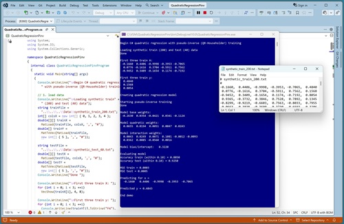 [Click on image for larger view.] Figure 1: Quadratic Regression with Pseudo-Inverse Training in Action.
The demo concludes by evaluating the trained model and making a prediction:
Evaluating model
Accuracy train (within 0.10) = 0.8850
Accuracy test (within 0.10) = 0.9250

MSE train = 0.0003
MSE test = 0.0005

Predicting for x =
  -0.1660   0.4406  -0.9998  -0.3953  -0.7065
Predicted y = 0.4843
The model accuracy is quite good compared to many other regression techniques applied to the synthetic dataset. The model achieves 88.50% accuracy on the training data (177 out of 200 correct) and 92.50% accuracy on the test data (37 out of 40 correct). A prediction is scored as correct if it's within 10% of the true target value.
This article assumes you have intermediate or better programming skill but doesn't assume you know anything about quadratic regression or pseudo-inverse training. The demo is implemented using C# but you should be able to refactor the demo code to another C-family language if you wish. All normal error checking has been removed to keep the main ideas as clear as possible.
The source code for the demo program is too long to be presented in its entirety in this article. The complete code and data are available in the accompanying file download, and they're also available online.
The Demo Data
The demo data is synthetic. It was generated by a 5-10-1 neural network with random weights and bias values. The idea here is that the synthetic data does have an underlying, but complex, non-linear structure which can be predicted.
All of the predictor values are between -1 and +1. When using quadratic regression, technically, it's not necessary to normalize/scale your data. But normalized data is easier to train and can lead to a better prediction model, especially if some raw predictor values are very large (such as employee salary) and some values are small (such as employee age). Also, using normalized data allows you to interpret the model weights more easily (larger magnitudes have more effect on the predicted y value).
Quadratic regression is most often used with data that has strictly numeric predictor variables. It is possible to use the technique with categorical data that has an inherent order using equal-interval encoding. For example, a predictor variable competence with possible values (low, medium, high) could be encoded as low = 0.25, medium = 0.50, high = 0.75.
However, for categorical data without inherent order, such as eye-color with possible values (brown, blue, green), there's no obvious way to encode the values so that when multiplied with other predictor values you get a meaningful number. That said, I have seen examples where non-ordered categorical predictor values were equal-interval encoded and the resulting prediction model worked quite well. But there are no solid research results, which I'm aware of, that support this encoding technique for quadratic regression.
Understanding Quadratic Regression
Suppose, as in the demo data, there are five predictors, (x0, x1, x2, x3, x4). The prediction equation for basic linear regression is:
y' = (w0 * x0) + (w1 * x1) + (w2 * x2) + (w3 * x3) + (w4 * x4) + b
The wi are model weights (aka coefficients), and b is the model bias (aka intercept). The values of the weights and the bias must be determined by training, so that predicted y' values are close to the known, correct y values in a set of training data.
Basic linear regression is simple but it can't predict well for data that has an underlying non-linear structure. Also, basic linear regression can't deal with data that has hidden interactions between the xi predictors.
The prediction equation for quadratic regression with five predictors is:
y' = (w0 * x0) + (w1 * x1) + (w2 * x2) + (w3 * x3) + (w4 * x4) +

     (w5 * x0*x0) + (w6 * x1*x1) + (w7 * x2*x2) +
     (w8 * x3*x3) + (w9 * x4*x4) +

     (w10 * x0*x1) + (w11 * x0*x2) + (w12 * x0*x3) + (w13 * x0*x4) +
     (w14 * x1*x2) + (w15 * x1*x3) + (w16 * x1*x4) +
     (w17 * x2*x3) + (w18 * x2*x4) +
     (w19 * x3*x4)

     + b
The squared ("quadratic") xi^2 terms handle non-linear structure. If there are n predictors, there are also n squared terms. The xi * xj terms between all possible pairs of original predictors handle interactions between predictors. If there are n predictors, there are (n * (n-1)) / 2 interaction terms.
Therefore, in general, if there are n original predictor variables, there are a total of n + n + (n * (n-1))/2 model weights and one bias. Behind the scenes, when using pseudo-inverse training, it's necessary to create an explicit augmented dataset with the derived variables, because all the values must be in a matrix. Despite the multiplication of the base predictors, the model is still a linear model in mathematical terms.
After training, to make a prediction for new, previously unseen data, the derived xi^2 squared terms and the derived xi*xj interactions terms can be computed programmatically on-the-fly.
Quadratic regression is a subset of what is called polynomial regression. For example, cubic regression includes xi^3 terms, quartic regression includes xi^4, and so on. In practice, it's rare to go beyond quadratic regression, in part because the number of derived predictors increases very quickly. For example, for the demo data with just 5 predictors, cubic regression has 55 derived predictor variables, and quartic regression has 125 derived variables.
Quadratic regression is a superset of linear regression with two-way interactions. Linear regression with two-way interactions includes only the derived xi * xj terms, and omits the xi^2 terms.
Quadratic regression might seem strange if you're new to the technique. Suppose you have a predictor x0 = employee-age and a predictor x1 = employee-income. The x0 * x1 term has no physical meaning -- it's just a new math predictor variable that can deal with hidden interactions between age and income.
Understanding Training Using Pseudo-Inverse
In theory, the weight values of a quadratic regression model can be solved using the equation w = inv(DX) * y, where w is the vector of weights and the bias that you want, DX is a "design matrix", which is a matrix of training predictor data that has a leading column of 1.0 values prepended, inv() is the regular matrix inverse operation, * means matrix-to-vector multiplication, and y is a vector of the target y values. However, this equation won't work because matrix inverse applies only to square matrices that have the same number of rows and columns. This is almost never the case in machine learning scenarios.
One workaround is to use what's called the relaxed Moore-Penrose pseudo-inverse. The math equation is w = pinv(DX) * y. This technique works because the pseudo-inverse applies to any shape matrix.
The code for pseudo-inverse training is short but a bit deceptive because most of the work is done by helper functions:
public void Train(double[][] trainX, double[] trainY)
{
  int dim = trainX[0].Length;
  int nInteractions = (dim * (dim - 1)) / 2;
  this.weights = new double[dim + dim + nInteractions];
  double[][] X = MatDesign(trainX);  // design X
  double[][] Xpinv = MatPseudoInv(X); // QR version
  double[] biasAndWts = MatVecProd(Xpinv, trainY);
  this.bias = biasAndWts[0];  // bias is at [0]
  for (int i = 1; i < biasAndWts.Length; ++i)
    this.weights[i - 1] = biasAndWts[i];
}
A design matrix takes the bias into account. For example, if a set of training predictors stored in a matrix X is:
0.80  0.07  0.62
0.22  0.71  0.14
0.94  0.03  0.73
The associated design matrix is:
1.0  0.80  0.07  0.62
1.0  0.22  0.71  0.14
1.0  0.94  0.03  0.73
OK, so what is needed is a function to compute the pseudo-inverse of a matrix. Unfortunately, implementing a pseudo-inverse function is very difficult. Many mathematicians worked for many years on the problem, and came up with dozens of solutions. The technique used by the demo program is to compute the pseudo-inverse of a matrix using QR decomposition via the Householder algorithm.
The good news is that the demo MatPseudoInv() pseudo-inverse function and its associated MatDecomposeQR() helper function can be considered black boxes. You won't have to modify the code except in very rare situations. The bad news is that because pseudo-inverse is complicated, it can fail due to numerical instability related to arithmetic overflow or underflow. But in practice, pseudo-inverse failure is very rare. The chance of failure increases as the size of the set of training data increases. As a crude rule of thumb, pseudo-inverse training for linear regression usually works well when the number of training items is less than 2,000.
For a source matrix A, the QR decomposition is A = Q * R. Taking the inverse of both side of the equation gives inv(A) = inv(Q * R), which simplifies to Ainv = inv(R) * inv(Q). The R matrix is square upper triangular (zeros below the main diagonal) and it's possible to compute the inverse for this special case easily. The inverse of the Q matrix is the transpose of Q (rows and columns switched), which is also easy to compute.
To recap, to train a quadratic regression model, you compute the pseudo-inverse of the design matrix and multiply it by a vector of target y values. To get the pseudo-inverse of the design matrix, you compute the QR decomposition and then easily compute the inverses of the resulting Q and R matrices, and then matrix-multiply those inverses together.
Alternatives to Pseudo-Inverse Training
An alternative to relaxed Moore-Penrose pseudo-inverse training for quadratic regression is stochastic gradient descent (SGD) training. SGD training estimates the values of the weights and bias using an iterative technique that starts with random values, and then slowly adjusts the weights and bias to get closer and closer to the optimal values. SGD requires a learning rate parameter that controls how quickly the values of the weights change, and a maximum iterations parameter that specifies how many iterations to perform. These two parameters must be determined by trial and error.
A second alternative to using relaxed Moore-Penrose pseudo-inverse training via QR decomposition is called left pseudo-inverse via normal equations closed form training. The equation for this training is w = inv(Xt * X) * Xt * y, where X is the design matrix, Xt is its transpose, inv() is regular matrix inverse (usually Cholesky inverse), * is matrix multiplication, and y is a vector of target values from the training data. This type of closed form training can fail for large matrices because the Xt * X operation uses many multiplications, and if the matrix values are very small or very large, arithmetic underflow or overflow can occur.
And to make things even more confusing, there is a true mathematical Moore-Penrose pseudo-inverse, which has rigorous math conditions, including solution uniqueness. The practical relaxed Moore-Penrose pseudo-inverse works well enough for machine learning scenarios.
The pseudo-inverse training used in the demo program uses QR decomposition with the Householder algorithm. QR decomposition can also be accomplished using the modified Gram-Schmidt algorithm or the Givens algorithm. All three QR decomposition algorithms are roughly equal in terms of effectiveness for training a quadratic regression model. Scientific applications that require a true Moore-Penrose pseudo-inverse with high precision use singular value decomposition (SVD). SVD is extremely complicated and is almost always overkill for machine learning scenarios where the emphasis is on prediction with noisy data.
To summarize, there are three common ways to train a quadratic regression model: stochastic gradient descent, relaxed Moore-Penrose pseudo-inverse (this article), left pseudo-inverse via normal equations. For very large datasets, using SGD is a good approach, but you must use trial and error to determine the learning rate and the maximum epochs. For medium size datasets, MP pseudo-inverse often works best. For small datasets, left pseudo-inverse training often works well. Note: There are many other training techniques, such as L-BFGS optimization and simplex optimization, but SGD, Moore-Penrose pseudo-inverse, and left pseudo-inverse are the most commonly used, at least based on my experience.
The Demo Program
I used Visual Studio 2026 (Community Free Edition) for the demo program. I created a new C# console application and checked the "Place solution and project in the same directory" option. I specified .NET version 10.0. I named the project QuadraticRegressionPinv. I checked the "Do not use top-level statements" option to avoid the strange program entry point shortcut syntax.
The demo has no significant .NET dependencies and any relatively recent version of Visual Studio with .NET (Core) or the older .NET Framework will work fine. You can also use the Visual Studio Code program if you like.
After the template code loaded into the editor, I right-clicked on file Program.cs in the Solution Explorer window and renamed the file to the more descriptive QuadraticRegressionPinvProgram.cs. I allowed Visual Studio to automatically rename class Program.
The overall program structure is presented in Listing 1. All the control logic is in the Main() method in the Program class. The Program class also holds helper functions to load data from file into memory and display data. All of the quadratic regression functionality is in a QuadraticRegressor class. The QuadraticRegressor class exposes a constructor and four methods: Train(), Predict(), Accuracy(), and MSE().
Listing 1: Overall Program Structure
using System;
using System.IO;
using System.Collections.Generic;

namespace QuadraticRegressionPinv
{
  internal class QuadraticRegressionPinvProgram
  {
    static void Main(string[] args)
    {
      Console.WriteLine("Begin C# quadratic regression" +
        " with pseudo-inverse (QR-Householder) training ");

      // 1. load data
      // 2. create and train model
      // 3. show model weights and bias
      // 4. evaluate trained model
      // 5. use model to make a prediction

      Console.WriteLine("End demo ");
      Console.ReadLine();
    } // Main

    // helpers for Main()
    static double[][] MatLoad(string fn, int[] usecols,
      char sep, string comment) { . . }

    static double[] MatToVec(double[][] M) { . . }

    static void VecShow(double[] vec, int dec, int wid) { . . }
  } // class Program

  // ========================================================

  public class QuadraticRegressor
  {
    public double[] weights;  // regular, quad, interactions
    public double bias;
    private Random rnd;  // not used w/ Pinv training

    public QuadraticRegressor(int seed = 0)  // ctor
    {
      this.weights = new double[0];  // empty, but not null
      this.bias = 0; // dummy value
      this.rnd = new Random(seed);
    }

    // core methods
    public void Train(double[][] trainX, double[] trainY) { . . }

    public double Predict(double[] x) { . . }

    public double Accuracy(double[][] dataX, double[] dataY,
      double pctClose) { . . }

    public double MSE(double[][] dataX, double[] dataY) { . . }

    // helpers for Train():
    private static double[][] MatDesign(double[][] trainX) { . . }

    private static double[] MatVecProd(double[][] M,
      double[] v) { . . }

    private static double[][] MatPseudoInv(double[][] M) { . . }

    private static void MatDecomposeQR(double[][] M,
      out double[][] Q, out double[][] R, bool reduced) { . . }

    private static double[][] MatInvUpperTri(double[][] U) { . . }

    // minor vector and matrix helpers
    private static double[][] MatCopy(double[][] M) { . . }
    private static double[][] MatTranspose(double[][] M) { . . }
    private static double[][] MatMake(int nRows, int nCols) { . . }
    private static double[][] MatIdentity(int n) { . . }
    private static double[][] MatProduct(double[][] A,
      double[][]B) { . . }
    private static double VecNorm(double[] vec) { . . }
    private static double VecDot(double[] v1, double[] v2) { . . }
    private static double[][] VecToMat(double[] vec, int nRows,
      int nCols) { . . }

  } // class QuadraticRegressor

  // ========================================================

} // ns
The QuadraticRegressor class declares the weights and bias class members with public scope so that they can be accessed directly to view them. The weights vector holds all the weights -- base weights, quadratic weights, and interaction weights. The 5 base weights are stored in cells [0] to [4]. The 5 quadratic weights are stored in cells [5] to [9]. The 10 interaction weights are stored in cells [10] to [19]. An alternative design is to use three separate vectors.
Loading the Data into Memory
The demo program starts by loading the 200-item training data into memory:
string trainFile =
  "..\\..\\..\\Data\\synthetic_train_200.txt";
int[] colsX = new int[] { 0, 1, 2, 3, 4 };
double[][] trainX =
  MatLoad(trainFile, colsX, ',', "#");
double[] trainY =
  MatToVec(MatLoad(trainFile,
  new int[] { 5 }, ',', "#"));
The training X data is stored into an array-of-arrays style matrix of type double. The data is assumed to be in a directory named Data, which is located in the project root directory. The arguments to the MatLoad() function mean load columns 0, 1, 2, 3, 4 where the data is comma-delimited, and lines beginning with "#" are comments to be ignored. The training y data in column [5] is loaded into a matrix and then converted to a one-dimensional vector using the MatToVec() helper function.
The 40-item test data is loaded into memory using the same pattern that was used to load the training data:
string testFile =
  "..\\..\\..\\Data\\synthetic_test_40.txt";
double[][] testX =
  MatLoad(testFile, colsX, ',', "#");
double[] testY =
  MatToVec(MatLoad(testFile,
  new int[] { 5 }, ',', "#"));
The first three training items are displayed with four decimals like so:
Console.WriteLine("First three train X: ");
for (int i = 0; i < 3; ++i)
  VecShow(trainX[i], 4, 8);
Console.WriteLine("First three train y: ");
for (int i = 0; i < 3; ++i)
  Console.WriteLine(trainY[i].ToString("F4").PadLeft(8));
In a non-demo scenario, you might want to display all the training data to make sure it was correctly loaded into memory.
Creating and Training the Model
The quadratic regression model is created and trained like so:
Console.WriteLine("Creating quadratic regression model ");
QuadraticRegressor model = new QuadraticRegressor();
Console.WriteLine("Starting pseudo-inverse training ");
model.Train(trainX, trainY);
Console.WriteLine("Done ");
The constructor accepts no parameters but has hidden a default seed value of 0 for the internal Random object. The Random object is not used by pseudo-inverse training, but it's in the QuadraticRegressor class in case you decide to add a second Train() method which needs a Random object.
After pseudo-inverse training is finished, the demo program displays the model base weights:
Console.WriteLine("Model base weights: ");
int dim = trainX[0].Length;
for (int i = 0; i < dim; ++i)
  Console.Write(model.weights[i].ToString("F4").PadLeft(8));
Console.WriteLine("");
And then displays the quadratic weights:
Console.WriteLine("Model quadratic weights: ");
for (int i = dim; i < dim + dim; ++i)
  Console.Write(model.weights[i].ToString("F4").PadLeft(8));
Console.WriteLine("");
And then the interaction weights and the bias:
Console.WriteLine("Model interaction weights: ");
for (int i = dim + dim; i < model.weights.Length; ++i) {
  Console.Write(model.weights[i].ToString("F4").PadLeft(8));
  if (i > dim+dim && i % dim == 0) Console.WriteLine("");
}
Console.WriteLine("");
Console.WriteLine("Model bias/intercept: " +
  model.bias.ToString("F4").PadLeft(8));
The demo program does not use any kind of explicit regularization, which is a technique that restricts the magnitude of the resulting model weights. Large model weights often lead to model overfitting when the model predicts well on the training data but poorly on new, previously unseen data. The most common way to apply regularization when using QR matrix decomposition is called Tikhonov regularization -- a topic outside the scope of this article.
Evaluating and Using the Model
The demo program evaluates the prediction accuracy of the trained model using these statements:
Console.WriteLine("Evaluating model ");
double accTrain = model.Accuracy(trainX, trainY, 0.10);
Console.WriteLine("Accuracy train (within 0.10) = " +
  accTrain.ToString("F4"));
double accTest = model.Accuracy(testX, testY, 0.10);
Console.WriteLine("Accuracy test (within 0.10) = " +
  accTest.ToString("F4"));
The Accuracy() method scores a prediction value as correct if it's within a specified percentage of the true target value. A reasonable closeness percentage to use will vary from problem to problem.
The model mean squared error (MSE) values are computed and displayed like so:
double mseTrain = model.MSE(trainX, trainY);
Console.WriteLine("MSE train = " + mseTrain.ToString("F4"));
double mseTest = model.MSE(testX, testY);
Console.WriteLine("MSE test = " + mseTest.ToString("F4"));
Mean squared error is a more granular metric than accuracy. MSE is useful when you want to compare two different models, for example, quadratic regression and nearest neighbors regression.
Another common evaluation metric is the coefficient of determination, R2. You can easily implement a coefficient of determination method by using the MSE() method as a template.
The demo concludes by using the trained model to predict the y value for the first training item, (-0.1660, 0.4406, -0.9998, -0.3953, -0.7065):
double[] x = trainX[0];
Console.WriteLine("Predicting for x = ");
VecShow(x, 4, 9);
double predY = model.Predict(x);
Console.WriteLine("Predicted y = " + predY.ToString("F4"));
The predicted y value, 0.4843, is very close to the true target value of 0.4840. This is an especially good result because the synthetic demo data was generated by a neural network, which has complex interactions between predictor variables.
Wrapping Up
Quadratic regression has a nice balance of prediction power and interpretability. The model weights/coefficients are easy to interpret. If the predictor values have been normalized to the same scale, larger magnitudes mean larger effect, and the sign of the weights indicate the direction of the effect. But you should be a bit careful interpreting the interaction weights. If an interaction weight is positive, it can indicate an increase in y when the corresponding pair of predictor values are both positive or both negative.
Quadratic regression is not always effective -- if it were, it would be used far more often than it is. Compared to basic linear regression, quadratic regression can sometimes provide a big improvement in model prediction accuracy for a relatively small investment in effort, and so it's usually worth exploring.