The Data Science Lab
Support Vector Regression with SGD Training Using C#
Support vector regression can predict numeric values effectively, and this article shows how to implement and train a kernel SVR model in C# using stochastic sub-gradient descent.
The goal of a machine learning regression problem is to predict a single numeric value. For example, a bank might want to predict the maximum safe loan amount for a customer, based on age, account balance, annual income, and so on.
There are approximately a dozen common regression techniques. Examples include linear regression, nearest neighbors regression, kernel ridge regression, tree-based regression (several types, such as random forest and gradient boosting), and neural network regression. Each technique has pros and cons. A technique that sometimes produces highly accurate predictions for specific types of data is called support vector regression (SVR).
The term "support vector regression" by itself is ambiguous, because there are two types of SVR: linear SVR and kernelized SVR. Linear SVR is rarely used so the term "SVR" by itself usually means kernel SVR. This article presents a demo of kernel SVR, trained using a variation of stochastic gradient descent (SGD) called stochastic sub-gradient descent (SSGD), with the radial basis function (RBF) hard-wired as the kernel function. Note: Even though SSGD is technically a variation of SGD, the two techniques are so similar that SSGD is often called SGD.
A good way to see where this article is headed is to take a look at the screenshot in Figure 1. The demo program begins by loading synthetic training and test data into memory. The data looks like:
-0.1660,  0.4406, -0.9998, -0.3953, -0.7065,  0.4840
 0.0776, -0.1616,  0.3704, -0.5911,  0.7562,  0.1568
-0.9452,  0.3409, -0.1654,  0.1174, -0.7192,  0.8054
 0.9365, -0.3732,  0.3846,  0.7528,  0.7892,  0.1345
. . .
The first five values on each line are the x predictors. The last value on each line is the target y variable to predict. There are 200 training items and 40 test items.
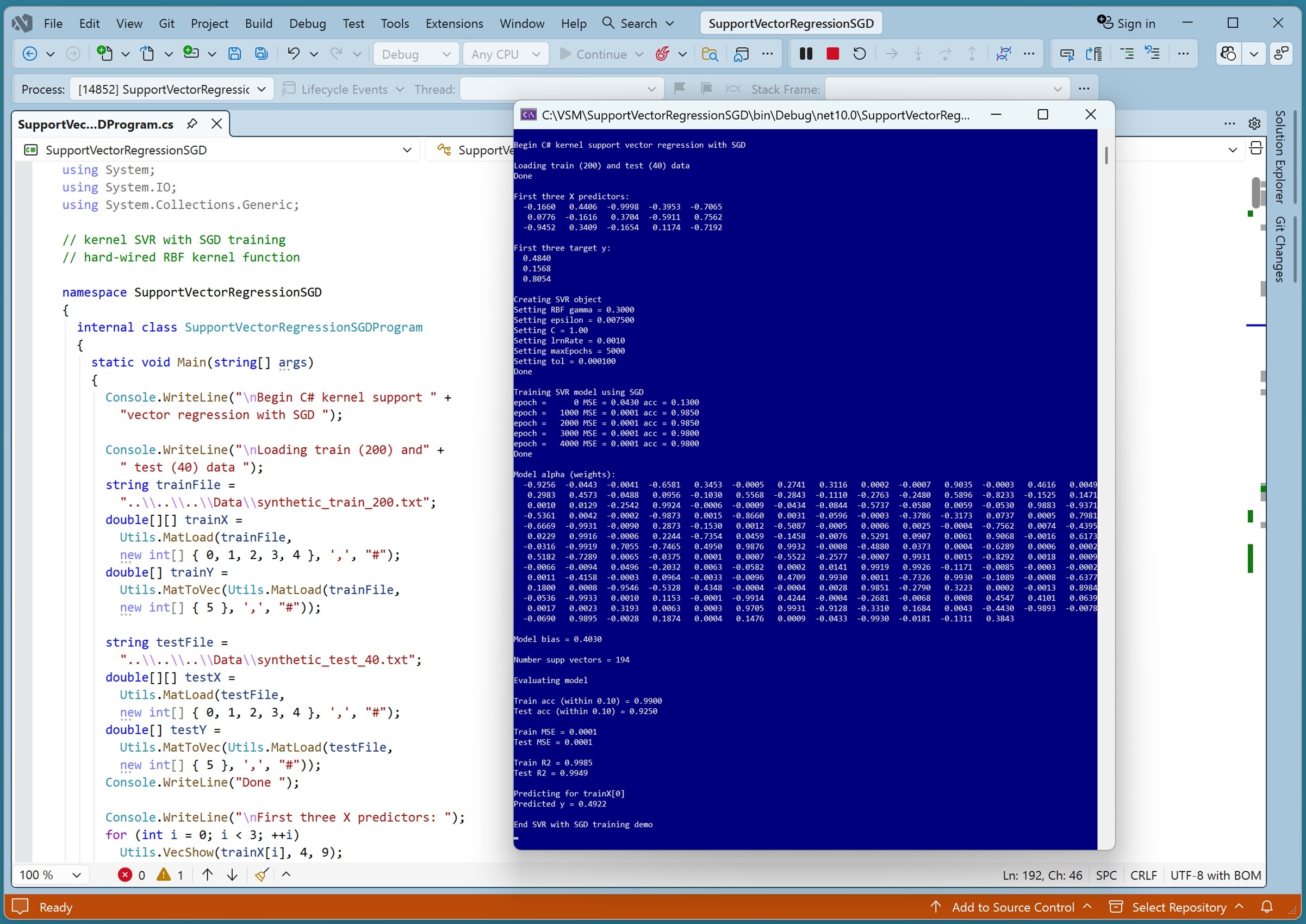 [Click on image for larger view.] Figure 1: Support Vector Regression with SGD Training in Action.
The demo creates and trains a kernel support vector regression model, evaluates the model accuracy on the training and test data, and then uses the model to predict the target y value for the first training item x = [-0.1660, 0.4406, -0.9998, -0.3953, -0.7065].
After displaying the first three training items, the demo shows how an SVR model is created and trained. The SVR parameters are displayed:
Creating SVR object
Setting RBF gamma = 0.3000
Setting epsilon = 0.007500
Setting C = 1.00
Setting lrnRate = 0.0010
Setting maxEpochs = 5000
Setting tol = 0.000100
The parameters will be explained shortly. One of the disadvantages of using SVR with SGD training is that it requires six parameters. The values for the six parameters must be determined by trial and error.
The SGD training technique is iterative. The demo uses 5,000 epochs (an epoch is one pass through all 200 training items) and displays progress messages every 1,000 epochs.
Training SVR model using SGD
epoch =      0 MSE = 0.0430 acc = 0.1300
epoch =   1000 MSE = 0.0001 acc = 0.9850
epoch =   2000 MSE = 0.0001 acc = 0.9850
epoch =   3000 MSE = 0.0001 acc = 0.9800
epoch =   4000 MSE = 0.0001 acc = 0.9800
Done
After training completes, the demo program displays the model weights and bias:
Model alpha (weights):
 -0.9256  -0.0443  -0.0041  -0.6581  . . .   0.0049
  0.2983   0.4573  -0.0488   0.0956  . . .   0.1471
. . .
  0.0017   0.0023   0.3193   0.0063  . . .  -0.0078
 -0.0690   0.9895   . . .    0.3843

Model bias = 0.4030
Number supp vectors = 194
During training, the SVR model computes one weight value into a vector called alpha for each training item, plus a special weight called the bias. During training, the SVR model determined that six of the 200 alpha weights were very close to zero, and so those six alpha values and their six associated training items were removed. This left 194 alpha weight values and training items, called the support vectors.
The demo program evaluates the trained model using three metrics:
Train acc (within 0.10) = 0.9900
Test acc (within 0.10) = 0.9250

Train MSE = 0.0001
Test MSE = 0.0001

Train R2 = 0.9985
Test R2 = 0.9949
The model scores 99.00 percent accuracy on the training data (198 out of 200 correct) and 92.50 percent accuracy on the test data (37 out of 40 correct). A prediction is scored as correct if it's within 10 percent of the true target value. The model mean squared error on both the training and test data is 0.0001, which is quite good. The model R2 score (also called the coefficient of determination) on the training data is 0.9985 and the R2 score on the test data is 0.9949. You can think of R2 as a normalized accuracy metric, and so the R2 scores are also quite good. In short, the SVR model predicts well.
The demo concludes with a sanity check by making a prediction for the first training item x = (-0.1660, 0.4406, -0.9998, -0.3953, -0.7065, 0.4840). The predicted y value is 0.4922, which is within 2 percent of the true target value of 0.4840.
This article assumes you have intermediate or better programming skills but doesn't assume you know anything about support vector regression. The demo is implemented using C#, but you should be able to refactor the demo code to another C-family language if you wish. All normal error checking has been removed to keep the main ideas as clear as possible.
The source code for the demo program is too long to be presented in its entirety in this article. The complete code and data are available in the accompanying file download, and they're also available at online.
The Demo Data
The demo data is synthetic. It was generated by a 5-10-1 neural network with random weights and bias values. The idea here is that the synthetic data does have an underlying, but complex, non-linear structure that can be predicted.
All of the predictor values are between -1 and +1. When using support vector regression, you should make sure that the data is normalized or scaled to roughly the same range. This prevents a predictor variable with large magnitude values (such as employee annual income) from overwhelming predictors with small magnitudes (such as employee age).
The three most common techniques to normalize numeric data are min-max normalization, z-score normalization, and divide-by-constant normalization. When possible, I recommend divide-by-constant normalization. For example, if you have a predictor variable employee age, you could divide all age values by 100.
Support vector regression is most often used with data that has strictly numeric predictor variables. It is possible to use the technique with categorical predictors. If a categorical predictor variable has an inherent order, you can use equal-interval encoding. For example, a predictor variable height with possible values (short, medium, tall) could be encoded as short = 0.25, medium = 0.50, tall = 0.75.
For categorical predictor variables without inherent order, such as employee-job with three possible values (sales, technical, management), you can use one-over-n-hot encoding. For instance, sales = (0.3333, 0, 0), technical = (0, 0.3333, 0), management = (0, 0, 0.3333). Unlike basic one-hot encoding, one-over-n-hot encoding takes into account the number of possible values of the predictor variable.
Understanding the RBF Kernel Function
Support vector regression requires a kernel function that computes the similarity between two vectors (training data items). The demo SVR system uses the radial basis function (RBF) as the kernel function.
There are two RBF versions that are mathematically equivalent: the gamma version and the sigma version. The RBF version used by the demo program is called the gamma version. The function is defined as:
rbf(v1, v2) = exp( -1 * gamma * ||v1 - v2||^2 )
Here, v1 and v2 are two vectors, exp() is the mathematical constant e (2.71828...) raised to a power, ||v1 -- v2||^2 is squared Euclidean distance, and gamma is an arbitrary constant. Gamma is sometimes called the inverse bandwidth, or just plain bandwidth, or scale.
Suppose v1 = (2.50, -3.25, 1.20) and v2 = (2.0, -3.0, 1.0) and gamma = 0.40. The trailing squared Euclidean distance term is the sum of the squared differences between vector elements:
||v1 - v2||^2 = (2.50 - 2)^2 + (-3.25 - (-3))^2 + (1.20 - 1)^2
              = (0.50)^2 + (-0.25)^2 + (0.20)^2
              = 0.2500 + 0.0625 + 0.0400
              = 0.3525
And then RBF(v1, v2) is:
rbf(v1, v2) = exp( -1 * gamma * ||v1 - v2||^2 )
            = exp( -1 * 0.40 * 0.3525 )
            = exp( -0.1410 )
            = 0.8685
If two vectors are the same, then rbf(v1, v2) = 1.0 (maximum similarity). The more different v1 and v2 are, the smaller the value of RBF is. Put another way, the RBF of two vectors is a value between 0 and 1 where larger values mean more similar.
There are many different kernel functions. In machine learning scenarios, the RBF kernel function is the most common (at least, based on my experience), and is the one used by the demo program. Other, less commonly used kernel functions include the polynomial kernel, the sigmoid kernel, and the cosine kernel.
Support Vector Regression Prediction
The support vector regression prediction mechanism is best understood by looking at a concrete example. In words, to predict the y value for an input vector x, you compute the sum of the products of the model alpha weights times the kernel function applied to x and each training item.
Suppose you have just four training data items, x0, x1, x2, x3. Suppose that during training, item x3 is removed, leaving three support vectors. A trained support vector regression model will have three alpha weights, a0, a1, a2. If the kernel function is the rbf() function, the predicted y for an input x is:
y' = (a0 * rbf(x, x0)) + (a1 * rbf(x, x1)) + (a2 * rbf(x, x2)) + bias
For example, suppose the input x to predict is (2.0, 4.0, 1.0). And suppose that for some value of gamma, the RBF kernel function values are:
rbf(x, x0) = 0.80
rbf(x, x1) = 0.50
rbf(x, x2) = 0.90
And suppose the trained model alpha weights are a0 = 0.60, a1 = 0.70, a2 = -0.20. If the model bias is 0.11, then the predicted y is:
y' = (a0 * rbf(x, x0)) + (a1 * rbf(x, x1)) + (a2 * rbf(x, x2)) + bias
   = (0.60 * 0.80) + (0.70 * 0.50) + (-0.20 * 0.90) + 0.11
   = (0.48 + 0.35 + -0.18) + 0.11
   = 0.65 + 0.11
   = 0.76
The demo Predict() method implementation, without error-checking, is short and simple:
public double Predict(double[] x)
{
  int n = this.suppX.Length;
  double sum = 0.0;
  for (int i = 0; i < n; ++i) {
    double[] sv = this.suppX[i];
    double k = this.RBF(x, sv);
    sum += this.wts[i] * k;
  }
  return sum + this.b;
}
The code uses suppX (support vectors X), which is the training X data after pruning. OK, but where do the model weights and the bias come from?
Training a Support Vector Regression Model
Training a support vector regression model is the process of finding values for the n model alpha weights (one per support vector) and the bias value so that predicted y values closely match the known correct target values in the training data.
There are three main ways to train a support vector regression model: quadratic programming (QP) optimization, the sequential minimal optimization (SMO) algorithm, and stochastic sub-gradient descent (SSGD / SGD). The demo uses SGD, which is the simplest SVR training technique.
Support vector regression uses the idea of an epsilon tube. Epsilon is a small value like 0.0001. The epsilon tube is a margin of tolerance around the predicted regression line / hyperplane, within which any deviation between the predicted and actual values is completely ignored and assigned zero error.
During training, alpha weights that are associated with data items that are in the epsilon tube are set to zero. Training items that predict too well are essentially removed by setting their weights to zero. The idea is not at all obvious -- items that predict too well don't add much value in theory so they can be removed.
The key code in the demo Train() method is:
double error = predY - trainY[idx];
bool insideTube = false;
if (error > this.epsilon) gradLoss = 1.0;
else if (error < -this.epsilon) gradLoss = -1.0;
else {
  gradLoss = 0.0;
  insideTube = true;
}
if (insideTube == true && Math.Abs(this.alpha[idx]) < this.tol)
  this.alpha[idx] = 0.0; // force to 0
After training has completed, the Train() method finds all the alpha weight values that are nearly 0, and removes them and the associated training vectors, leaving just the support vectors and support alpha weights.
The Demo Program
I used Visual Studio 2026 (Community Free Edition) for the demo program. I created a new C# console application and checked the "Place solution and project in the same directory" option. I specified .NET version 10.0. I named the project SupportVectorRegressionSGD. I checked the "Do not use top-level statements" option to avoid the strange program entry point shortcut syntax.
The demo has no significant .NET dependencies and any relatively recent version of Visual Studio with .NET (Core) or the older .NET Framework will work fine. You can also use the Visual Studio Code program if you like.
After the template code loaded into the editor, I right-clicked on the file Program.cs in the Solution Explorer window and renamed the file to the more descriptive SupportVectorRegressionSGDProgram.cs. I allowed Visual Studio to automatically rename the Program class.
The overall program structure is presented in Listing 1. All the control logic is in the Main() method in the Program class. All of the support vector regression functionality is in an SVR class. The SVR class exposes a constructor and five methods: Train(), Predict(), Accuracy(), MSE(), and R2(). The private RBF() method is used by the Train() and Predict() methods. The demo program has a utility class named Utils that contains static methods to load data from a text file into a matrix, compute a matrix inverse, and display data.
Listing 1: Overall Program Structure
using System;
using System.IO;
using System.Collections.Generic;

// kernel SVR with SGD training
// hard-wired RBF kernel function

namespace SupportVectorRegressionSGD
{
  internal class SupportVectorRegressionSGDProgram
  {
    static void Main(string[] args)
    {
      Console.WriteLine("Begin C# kernel support " +
        "vector regression with SGD ");

      // 1. load training and test data
      // 2. create and train model
      // 3. evaluate model
      // 4. use model to make a prediction

      Console.WriteLine("End SVR with SGD training demo ");
      Console.ReadLine();
    }
  }

  // ========================================================

  public class SVR
  {
    public double gamma;      // for RBF kernel
    public double epsilon;
    public double C;          // complexity regularization
    public double[][] suppX;  // needed for pred
    public double[] suppY;
    public double[] alpha;    // one per suppX item
    public double b;          // bias
    public double lrnRate;    // for SGD training
    public int maxEpochs;
    public double tol;        // defines a 0-alpha
    public Random rnd;

    // ------------------------------------------------------

    public SVR(double gamma, double epsilon, double C,
      double lrnRate, int maxEpochs, double tol,
      int seed = 0) { . . }

    public void Train(double[][] trainX, double[] trainY) { . . }

    private void Shuffle(int[] indices) { . . }
    private double RBF(double[] v1, double[] v2) { . . }
    private double[][] MakeK(double[][] X) { . . }

    public double Predict(double[] x) { . . }

    public double Accuracy(double[][] dataX,
      double[] dataY, double pctClose) { . . }

    public double MSE(double[][] dataX, double[] dataY) { . . }

    public double R2(double[][] dataX, double[] dataY) { . . }

  } // class KRR

  // ========================================================

  public class Utils
  {
    public static double[][] MatLoad(string fn,
      int[] usecols, char sep, string comment) { . . }

    public static double[] MatToVec(double[][] X) { . . }

     public static double[][] MatSelectRows(double[][] X,
      int[] rows) { . . }

    public static double[][] MatMake(int nRows, int nCols) { . . }

    public static double VecMean(double[] vec) { . . }

    public static int[] VecRange(int n)

    public static double[] VecSelectItems(double[] vec,
      int[] idxs) { . . }

    public static void VecShow(int[] vec, int wid) { . . }

    public static void VecShow(double[] vec, int dec, int wid) { . . }

    public static void MatShow(double[][] m, int dec, int wid) { . . }

  } // class Utils

} // ns
The SVR class declares its 11 fields with public scope so that they can be accessed directly. Unlike some regression techniques, support vector regression needs access to the X training predictor data because the Predict() method uses that data. The training data is saved as suppX and suppY ("support vectors X and support values Y").
Loading the Data into Memory
The demo program starts by loading the 200-item training data into memory:
string trainFile = "..\\..\\..\\Data\\synthetic_train_200.txt";
double[][] trainX = MatUtils.MatLoad(trainFile,
  new int[] { 0, 1, 2, 3, 4 }, ',', "#");
double[] trainY = MatUtils.MatToVec(MatUtils.MatLoad(trainFile,
  new int[] { 5 }, ',', "#"));
The training X data is stored into an array-of-arrays style matrix of type double. The data is assumed to be in a directory named Data, which is located in the project root directory. The arguments to the MatLoad() function mean to load columns 0, 1, 2, 3, 4 where the data is comma-delimited, and lines beginning with "#" are comments to be ignored. The training y data in column [5] is loaded into a matrix and then converted to a one-dimensional vector using the MatToVec() helper function.
The 40-item test data is loaded into memory using the same pattern that was used to load the training data:
string testFile = "..\\..\\..\\Data\\synthetic_test_40.txt";
double[][] testX = Utils.MatLoad(testFile,
  new int[] { 0, 1, 2, 3, 4 }, ',', "#");
double[] testY = Utils.MatToVec(Utils.MatLoad(testFile,
  new int[] { 5 }, ',', "#"));
The first three training items are displayed with four decimals like so:
Console.WriteLine("First three X predictors: ");
for (int i = 0; i < 3; ++i)
  Utils.VecShow(trainX[i], 4, 8);
Console.WriteLine("First three target y: ");
for (int i = 0; i < 3; ++i)
  Console.WriteLine(trainY[i].ToString("F4").PadLeft(8));
In a non-demo scenario, you might want to display all the training data to make sure it was correctly loaded into memory.
Creating and Training the Model
The support vector regression model is prepared by setting up six parameters:
double gamma = 0.30;
double epsilon = 0.0075;
double C = 1.0;
double lrnRate = 0.001;
int maxEpochs = 5000;
double tol = 1.0e-4;
All of the parameter values must be determined by trial and error. The gamma parameter defines the RBF function that is used to measure the similarity between data item vectors. Larger values of gamma shrink the radius of influence of individual training points. This tends to increase model accuracy at the expense of increased risk of model overfitting.
The epsilon value defines how close to correct a prediction must be to be considered a non-support vector or a support vector. Larger values of epsilon create fewer support vectors.
The C ("complexity") value is used for model regularization, which discourages model alpha weights from becoming very large, which often leads to model overfitting. Larger values of C increase model complexity (which usually decreases the number of support vectors), which usually increases model accuracy at the risk of increased model overfitting.
The lrnRate value controls how much alpha weight values change at each update during training. Larger values of lrnRate increase the speed of training, at the risk of jumping over good weight values.
The maxEpochs value controls how many iterations are performed during training. The effect of larger values of SVR maxEpochs can vary greatly.
The tol ("tolerance") value controls pruning away training vectors to support vectors, by defining how close to 0 an alpha weight value must be in order to be pruned away. Larger values of tol allow more alpha weights to be defined as zero, which reduces the number of support vectors.
The biggest weakness of support vector regression is the difficulty of tuning the hyperparameters. Small changes in parameter values can cause extremely large changes in the model, and the hyperparameters interact in complex ways. Based on my experience, I'd say that SVR is the most difficult regression technique to tune.
The SVR model is created and trained like so:
SVR model = new SVR(gamma, epsilon, C, lrnRate, maxEpochs, tol, seed: 0);
Console.WriteLine("Training SVR model using SGD ");
model.Train(trainX, trainY);
Console.WriteLine("Done ");
After training has completed, the demo program displays and analyzes the model alpha weights:
Console.WriteLine("Model alpha (weights): ");
Utils.VecShow(model.alpha, 4, 9);
Console.WriteLine("Model bias = " + model.b.ToString("F4"));
Console.WriteLine("Number supp vectors = " + model.suppX.Length);
Displaying the model weights and the bias values is generally a good idea to make sure the model doesn't have nearly all the same alpha weights, which indicates a problem with the model.
The demo computes three different model evaluation metrics:
double trainAcc = model.Accuracy(trainX, trainY, 0.10);
double testAcc = model.Accuracy(testX, testY, 0.10);

double trainMSE = model.MSE(trainX, trainY);
double testMSE = model.MSE(testX, testY);

double trainR2 = model.R2(trainX, trainY);
double testR2 = model.R2(testX, testY);
Model accuracy is usually what you are most interested in, and is the easiest metric to interpret. Model mean squared error is more granular than accuracy but more difficult to interpret. MSE varies depending on how training data is scaled. The model R2 score is sort of a normalized accuracy metric, where an R2 value of 1.0 is perfect model accuracy (not reachable in practice) and smaller R2 values, closer to 0.0, indicate worse accuracy. R2 values can be negative, which indicates the model predicts even worse than just predicting the average target y value for any input.
The demo concludes by using the trained model to predict the y value for the first training item, (-0.1660, 0.4406, -0.9998, -0.3953, -0.7065):
double[] x = trainX[0];
Console.WriteLine("Predicting for trainX[0] ");
double y = model.Predict(x);
Console.WriteLine("Predicted y = " + y.ToString("F4"));
The predicted y value, 0.4922, is reasonably close to the true target value of 0.4840. This is a good result considering that the synthetic demo data was generated by a neural network, which has complex interactions between predictor variables.
In some scenarios, you might want to save the trained model alpha weights so that the model can be used by other systems. The easiest way to do this is to implement a SaveWeights() method that writes a single line of comma-delimited model alpha weight values to a specified text file. The weights can be loaded by implementing a LoadWeights() method. Because support vector regression prediction requires the training/support data items, you'd need to save them too.
Wrapping Up
The first versions of kernelized support vector regression in the 1980s required quadratic programming optimization training, which is very complicated, slow, and doesn't scale well to large datasets. The sequential minimal optimization (SMO) training algorithm was developed in the late 1990s. SMO is fast but the algorithm is complicated, and very difficult to correctly implement. The SGD (actually stochastic sub-gradient descent, SSGD) training technique presented in this article is by far the simplest training algorithm, and often works well in practice because processing one data item at a time introduces a form of implicit regularization, which helps the SVR model to predict new, previously unseen data.
Support vector regression had a brief surge of popularity in the late 1990s and early 2000s. However, data scientists realized that the closely related kernel ridge regression (KRR) has several significant advantages over SVR, and so the use of SVR declined to the point where it is not used very much today. SVR is more difficult to implement than KRR, SVR is much more difficult to tune than KRR (KRR can use true SGD, which is easier to tune than SVR sub-gradient descent), and SVR often gives slightly worse prediction accuracy than KRR (due mostly to the difficulty in parameter tuning). That said, there are some problem domains, such as biology and chemistry, where kernel SVR is often used and is highly effective.