The Data Science Lab
Logistic Regression Using the scikit Library
Dr. James McCaffrey of Microsoft Research says the main advantage of scikit is that it's easy to use (even though most classes have many constructor parameters).
Logistic regression is a machine learning technique for binary classification. For example, you might want to predict the sex of a person (male or female) based on their age, state where they live, income and political leaning. There are many other techniques for binary classification, but logistic regression was one of the earliest developed and the technique is considered a fundamental machine learning skill for data scientists.
There are many tools and code libraries that you can use to perform logistic regression. The scikit-learn library (also called scikit or sklearn) is based on the Python language and is one of the most popular machine learning libraries.
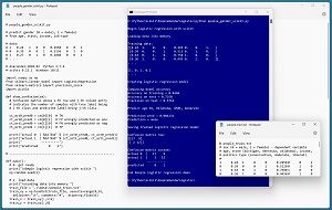
A good way to see where this article is headed is to take a look at the screenshot in Figure 1. The demo program loads a 200-item set training data, and a 40-item set of test data into memory. Next, the demo creates and trains a logistic regression model using the LogisticRegression class from the scikit library.
 [Click on image for larger view.] Figure 1: Logistic Regression Using scikit in Action/figcaption>
After training, the model is applied to the training data and the test data. The model scores 84.50 percent accuracy (169 out of 200 correct) on the training data, and 72.50 percent accuracy (29 out of 40 correct) on the test data.
The demo uses the trained model to make a gender prediction for a new, previously unseen person. The new person is age 36, from Oklahoma, has an income of $50,000 and is a political moderate. The raw p-value output is 0.0043 and because the p-value is less than 0.5 the prediction is class 0 = male. If the p-value had been greater than 0.5 then the prediction would have been class 1 = female.
The demo concludes by displaying a confusion matrix that shows the counts of the four possible outcomes for a binary classification problem. The counts are: the number of class 0 (male) correctly predicted (17), the number of class 0 incorrectly predicted (9), the number of class 1 (female) incorrectly predicted (2) and the number of class 1 correctly predicted (12).
This article assumes you have intermediate or better skill with a C-family programming language, but doesn't assume you know much about logistic regression or the scikit library. The complete source code for the demo program is presented in this article. The source code is also available in the accompanying file download and also online.
Installing the scikit Library
There are several ways to install the scikit library. I recommend installing the Anaconda Python distribution. Anaconda contains a core Python engine plus over 500 libraries that are (mostly) compatible with each other. I used Anaconda3-2020.02 which contains Python 3.7.6 and the scikit 0.22.1 version. The demo code runs on Windows 10 or 11.
Briefly, Anaconda is installed using a Windows self-extracting executable file. The setup process is mostly straightforward and takes about 15 minutes. You can consult step-by-step instructions.
There are more up-to-date versions of Anaconda/Python/scikit library available. But because the Python ecosystem has hundreds of libraries, if you install the most recent versions of these libraries, you run a greater risk of library incompatibilities -- a major headache when working with Python.
The Data
The data, available here, is artificial. The structure of data looks like:
1   0.24   1   0   0   0.2950   0   0   1
0   0.39   0   0   1   0.5120   0   1   0
1   0.63   0   1   0   0.7580   1   0   0
0   0.36   1   0   0   0.4450   0   1   0
1   0.27   0   1   0   0.2860   0   0   1
. . .
The tab-delimited fields are sex (0 = male, 1 = female), age (divided by 100), state (Michigan = 100, Nebraska = 010, Oklahoma = 001), income (divided by $100,000) and political leaning (conservative = 100, moderate = 010, liberal = 001). For scikit logistic regression, the variable to predict should be encoded as 0 or 1. The numeric predictors should be normalized to all the same range, typically 0.0 to 1.0 or -1.0 to +1.0. The categorical predictors should be one-hot encoded. For example, if there were five states instead of just three, the states would be encoded as 10000, 01000, 00100, 00010, 00001.
Understanding How Logistic Regression Works
Understanding how logistic regression works is best explained by example. Suppose, as in the demo program, the goal is to predict the sex of a person who is 36 years old, lives in Oklahoma, makes $50,000 and who is a political moderate. Each input variable has an associated numeric weight value, and there is a special weight called a bias. Suppose the model weights are [79.3, 1.8, 1.8, 0.3, -78.6, 3.8, 1.1, -1.0] and the bias is 3.9.
The first step is to sum the products of each input variable and its associated weight, and then add the bias:
z = (0.36)(79.3) +
    (0)(1.8) + (0)(1.8) + (1)(0.3) +
    (0.5000)(-78.6) +
    (0)(3.8) + (1)(1.1) + (0)(-1.0) +
    (3.9)
  = -5.45
The next step is to compute a p-value:
p = 1 / (1 + exp(-z))
  = 1 / (1 + exp(+5.45))
  = 0.0043
The computed p-value will always be between 0 and 1. The last step is to interpret the p-value. If the computed p-value is less than 0.5, the prediction is class 0 (male), and if the computed p-value is greater than 0.5, the prediction is class 1 (female).
The Demo Program
The complete demo program is presented in Listing 1. I am not ashamed to admit that Notepad is my preferred code editor, but most of my colleagues use a more sophisticated programing environment. I indent my Python program using two spaces rather than the more common four spaces.
The program imports the NumPy library, which contains numeric array functionality. The LogisticRegression module has the key code for performing logistic regression. Notice the name of the root scikit module is sklearn rather than scikit.
The precision_score module contains code to compute precision -- a special type of accuracy for binary classification. The pickle library has code to save a trained model. (The word pickle means to save food for later use, as in pickled cucumbers.)
Listing 1: Complete Demo Program
# people_gender_scikit.py

# predict gender (0 = male), 1 = female)
# from age, state, income, job-type

# data:
# 1   0.24   1   0   0   0.2950   0   0   1
# 0   0.39   0   0   1   0.5120   0   1   0
# 1   0.27   0   1   0   0.2860   0   0   1
# . . .

# Anaconda3-2020.02  Python 3.7.6
# scikit 0.22.1  Windows 10/11

import numpy as np
from sklearn.linear_model import LogisticRegression
from sklearn.metrics import precision_score
import pickle

def show_confusion(cm):
  # Confusion matrix whose i-th row and j-th column entry
  # indicates the number of samples with true label being
  # i-th class and predicted label being j-th class.

  ct_act0_pred0 = cm[0][0]  # TN
  ct_act0_pred1 = cm[0][1]  # FP wrongly predicted as pos
  ct_act1_pred0 = cm[1][0]  # FN wrongly predicted as neg
  ct_act1_pred1 = cm[1][1]  # TP

  print("actual 0  | %4d %4d" % (ct_act0_pred0, ct_act0_pred1))
  print("actual 1  | %4d %4d" % (ct_act1_pred0, ct_act1_pred1))
  print("           ----------")
  print("predicted      0    1")

# -----------------------------------------------------------

def main():
  # 0. get ready
  print("\nBegin logistic regression with scikit ")
  np.random.seed(1)

  # 1. load data
  print("\nLoading data into memory ")
  train_file = ".\\Data\\people_train.txt"
  train_xy = np.loadtxt(train_file, usecols=range(0,9),
    delimiter="\t", comments="#",  dtype=np.float32)
  train_x = train_xy[:,1:9]
  train_y = train_xy[:,0]

  test_file = ".\\Data\\people_test.txt"
  test_xy = np.loadtxt(test_file, usecols=range(0,9),
    delimiter="\t", comments="#",  dtype=np.float32)
  test_x = test_xy[:,1:9]
  test_y = test_xy[:,0]

  print("\nTraining data:")
  print(train_x[0:4])
  print(". . . \n")
  print(train_y[0:4])
  print(". . . ")

  # 2. create model and train
  print("\nCreating logistic regression model")
  model = LogisticRegression(random_state=0,
    solver='sag', max_iter=1000, penalty='none')
  model.fit(train_x, train_y)

  # 3. evaluate
  print("\nComputing model accuracy ")
  acc_train = model.score(train_x, train_y)
  print("Accuracy on training = %0.4f " % acc_train)

  acc_test = model.score(test_x, test_y)
  print("Accuracy on test = %0.4f " % acc_test)

  y_predicteds = model.predict(test_x)
  precision = precision_score(test_y, y_predicteds)
  print("Precision on test = %0.4f " % precision)

  # 4. make a prediction
  print("\nPredict age 36, Oklahoma, $50K, moderate ")
  x = np.array([[0.36, 0,0,1, 0.5000, 0,1,0]],
    dtype=np.float32)

  p = model.predict_proba(x)
  p = p[0][1]  # first (only) row, second value P(1)

  print("\nPrediction prob = %0.6f " % p)
  if p  < 0.5:
    print("Prediction = male ")
  else:
    print("Prediction = female ")

  # 5. save model
  print("\nSaving trained logistic regression model ")
  path = ".\\Models\\people_scikit_model.sav"
  pickle.dump(model, open(path, "wb"))

  # 6. confusion matrix with labels
  from sklearn.metrics import confusion_matrix
  cm = confusion_matrix(test_y, y_predicteds)
  print("\nConfusion matrix raw: ")
  print(cm)

  print("\nConfusion matrix custom: ")
  show_confusion(cm)

  print("\nEnd People logistic regression demo ")

if __name__ == "__main__":
  main()
The demo begins by setting the NumPy random seed:
def main():
  # 0. get ready
  print("Begin logistic regression with scikit ")
  np.random.seed(1)
. . .
Technically, setting the random seed value isn't necessary, but doing so allows you to get reproducible results in most situations.
Loading the Training and Test Data
The demo program loads the training data into memory using these statements:
  # 1. load data
  print("Loading data into memory ")
  train_file = ".\\Data\\people_train.txt"
  train_xy = np.loadtxt(train_file, usecols=range(0,9),
    delimiter="\t", comments="#",  dtype=np.float32)
  train_x = train_xy[:,1:9]
  train_y = train_xy[:,0]
This code assumes the data files are stored in a directory named Data. There are many ways to load data into memory. I prefer using the NumPy library loadtxt() function but a common alternative is the Pandas library read_csv() function.
The code reads all 200 lines of training data (columns 0 to 8 inclusive) into a matrix named train_xy and then splits the data into a matrix of predictor values and a vector of target gender values. The colon syntax means "all rows."
The 40-item test data is read into memory in the same way as the training data:
  test_file = ".\\Data\\people_test.txt"
  test_xy = np.loadtxt(test_file, usecols=range(0,9),
    delimiter="\t", comments="#",  dtype=np.float32)
  test_x = test_xy[:,1:9]
  test_y = test_xy[:,0]
The demo program prints the first four predictor items and the first four target gender values:
  print("Training data:")
  print(train_x[0:4])
  print(". . . \n")
  print(train_y[0:4])
  print(". . . ")
In a non-demo scenario you might want to display all the training data.
Creating and Training the Model
Creating and training the logistic regression model is simultaneously simple and complicated:
  print("Creating logistic regression model")
  model = LogisticRegression(random_state=0,
    solver='sag', max_iter=1000, penalty='none')
  model.fit(train_x, train_y)
Like most scikit models, the LogisticRegression class has a lot of parameters:
LogisticRegression(penalty='l2', *, dual=False, tol=0.0001, C=1.0, fit_intercept=True, intercept_scaling=1, class_weight=None, random_state=None, solver='lbfgs', max_iter=100, multi_class='auto', verbose=0, warm_start=False, n_jobs=None, l1_ratio=None)
When working with scikit, you'll spend most of your time reading the documentation and trying to figure out what each parameter does. The random_state parameter sets the seed value for an internal random number generator that shuffles the order of the training data during training.
The solver parameter is set to 'sag' (stochastic average gradient). There are five other solver algorithms, but the most common, and the default, is 'lbgs' (limited-memory Broyden-Fletcher-Goldfarb-Shanno). The 'lbfgs' algorithm works well with relatively small datasets but 'sag' often works better with large datasets.
The max_iter value is one parameter that requires a lot of trial and error. If you train too many iterations, you can overfit where accuracy is good on training data but poor on test data. If you train too few iterations, you will underfit and get poor accuracy on training and test data.
The penalty parameter is set to 'none'. For the 'sag' solver the only two options are 'none' and 'l2' (also called ridge regression). The L2 penalty discourages model weights from becoming very large. Note that in scikit versions 1.2 and newer you'd use None (no quotes) instead of 'none'.
After everything has been prepared, the model is trained using the fit() method. Almost too easy.
Evaluating the Trained Model
The demo computes the accuracy of the trained model like so:
  print("Computing model accuracy ")
  acc_train = model.score(train_x, train_y)
  print("Accuracy on training = %0.4f " % acc_train)
  acc_test = model.score(test_x, test_y)
  print("Accuracy on test = %0.4f " % acc_test)
The score() function computes a simple accuracy, which is just the number of correct predictions divided by the total number of predictions. However, for binary classification problems, you almost always want additional evaluation metrics due to the possibility of unbalanced data. Suppose the 200-item training data had 180 males and 20 females. A model that predicts male for any set of inputs would always achieve 180 / 200 = 90 percent accuracy.
Three common evaluation metrics that provide additional information are precision, recall and F1 score. The demo computes precision:
  y_predicteds = model.predict(test_x)
  precision = precision_score(test_y, y_predicteds)
  print("Precision on test = %0.4f " % precision)
The scikit library also has a recall_score() and an f1_score() function. In general you should compute precision and recall and only be concerned when either is very low. The F1 score metric is just the harmonic mean of precision and recall.
Using the Trained Model
The demo program uses the model to predict the sex of a new, previously unseen person:
  print("Predict age 36, Oklahoma, $50K, moderate ")
  x = np.array([[0.36, 0,0,1, 0.5000, 0,1,0]],
    dtype=np.float32)
  p = model.predict_proba(x)
  p = p[0][1]  # first (only) row, second value P(1)

  print("Prediction prob = %0.6f " % p)
  if p  < 0.5:
    print("Prediction = male ")
  else:
    print("Prediction = female ")
Because the logistic regression model was trained using normalized and encoded data, the x-input must be normalized and encoded in the same way. Notice the double square brackets on the x-input. The predict_proba() function expects a matrix rather than a vector.
The return result from the predict_proba() function ("probabilities array") has only one row because only one input was supplied. The two values in the row are the probabilities of class 0 and class 1, respectively. It's common to use just the probability of class 1 so that values less than 0.5 indicate a prediction of class 0 and values greater than 0.5 indicate a prediction of class 1.
Saving the Trained Model
The trained model is saved like so:
  print("Saving trained logistic regression model ")
  path = ".\\Models\\people_scikit_model.sav"
  pickle.dump(model, open(path, "wb"))
This code assumes there is a directory named Models. A saved model could be loaded from another program like so:
  # age 28, Nebraska, $62K, conservative
  x = np.array([[0.28, 0,1,0, 0.6200, 1,0,0]],
    dtype=np.float32)
  with open(path, 'rb') as f:
    loaded_model = pickle.load(f)
  pa = loaded_model.predict_proba(x)
  print(pa)
There are several other ways to save and load a trained scikit model, but using the pickle library is simplest.
Displaying and Understanding a Confusion Matrix
The demo program displays the trained model's results for the 40-item test data in a confusion matrix:
  from sklearn.metrics import confusion_matrix
  y_predicteds = model.predict(test_x)
  cm = confusion_matrix(test_y, y_predicteds)
  print("Confusion matrix raw: ")
  print(cm)
The output looks like:
  [[17  9]
   [ 2 12]]
The top row values are for actual data is class 0. Therefore, there are 17 (actual = class 0 and predicted = class 0), called true negatives. There are 9 (actual = 0 and predicted = 1), called false positives. There are 2 (actual = 1 and predicted 0), called false negatives. And there are 12 (actual = 1 and predicted = 1), called true positives.
The demo implements a program-defined show_confusion() function that takes the output from the built-in confusion_matrix() and adds some labels to make the output easier to understand.
Wrapping Up
Using the scikit library is a good option for many simple machine learning algorithms. The main advantage of scikit is that it's easy to use. In particular the fit() function for all types of models just works without any fuss. The primary disadvantage of scikit in my opinion is that the constructor for most models has a lot of parameters and so you must spend a lot of time wading through documentation.