Neural Network Lab
Use Python with Your Neural Networks
A neural network implementation can be a nice addition to a Python programmer's skill set. If you're new to Python, examining a neural network implementation is a great way to learn the language.
One of the most common requests I get from readers is to demonstrate a neural network implemented using the Python programming language. The use of Python appears to be increasing steadily. If you currently use Python, adding a neural network implementation can be a valuable addition to your skill set. If you don't know Python, examining the implementation presented in this article is a great way to get up to speed with the language.
The best way to get a feel for where this article is headed is to take a look at Figure 1, which shows a demonstration of a Python program predicting the species of an iris flower based on the flower's color (blue, pink or teal), petal length and petal width. The raw data resembles:
 [Click on image for larger view.]
Figure 1. Python Neural Network in Action
[Click on image for larger view.]
Figure 1. Python Neural Network in Action
blue, 1.4, 0.3, setosa
pink, 4.9, 1.5, versicolor
teal, 5.6, 1.8, virginica
The three predictor variables -- color, length and width -- are in the first three columns and the dependent variable, species (setosa, versicolor or virginica) is in the fourth column. The demo data is artificial, but is based on the well-known Fisher's Iris benchmark data set. The demo sets up a 24-item set of training data, used to create the model, and a six-item set of test data, used to estimate the accuracy of the model.
The non-numeric data in the training and test sets (color and species) has been encoded. Color uses 1-of-(N-1) encoding so that blue is (1, 0), pink is (0, 1) and teal is (-1, -1). Species uses 1-of-N encoding so that setosa is (1, 0, 0), versicolor is (0, 1, 0) and virginica is (0, 0, 1). For simplicity, the numeric data (petal length and width) was not normalized because their magnitudes are all roughly the same, so neither would dominate the other.
The demo creates a neural network with four input nodes (one for each predictor value), five hidden processing nodes (found by trial and error) and three output nodes (one for each species-value). The demo neural network uses the hyperbolic tangent function for hidden node activation, and uses the softmax activation function for output node activation.
The demo program trains the neural network using an artificial technique of randomly guessing values for the (numInput * numHidden) + numHidden + (numHidden * numOutput) + numOutput = (4 * 5) + 5 + (5 * 3) + 3 = 43 weights and bias values. I will present a Python implementation of the back-propagation training algorithm in the next Neural Network Lab column.
After the pseudo-training completes, the demo program displays the best set of 43 weights and bias values found. Using these values, the neural network correctly predicts the species of 75.00 percent of the training data (18 out of 24 correct; actually, not too bad considering that training was random guesses) and 66.67 percent (4 out of 6 correct) on the test data.
This article assumes you have a basic familiarity with neural networks but doesn't assume you know anything about Python programming. The demo program is a bit too long to present in its entirety in this article, but the complete source code is available in the accompanying code download.
Although there are several existing open source Python implementations available, in my opinion, the learning curve required for using a neural network library written by someone else is quite high. Writing a neural network from scratch gives you a complete understanding of your code base and allows you to keep the code simple when appropriate and customize when necessary.
Overall Program Structure
The overall structure of the demo program, with a few minor edits to save space, is presented in Listing 1. To create the demo, I first installed Python from python.org. I used the older version 2.7 rather than the current version 3 because the newer version is not entirely backward-compatible and many of my colleagues still use the 2.x versions. I accepted all the installation default values.
Listing 1: Overall Program Structure
# neuralnetweaktrain.py
# uses Python version 2.7
# weak training by randomly guessing

import random
import math

# ------------------------------------

def showdata(matrix, numFirstRows): . . .
def showvector(vector): . . .

# ------------------------------------

class NeuralNetwork: . . .

# ------------------------------------

print "Begin neural network using Python"
print "Goal is to predict species\n"
print "Raw data looks like: \n"
print "blue, 1.4, 0.3, setosa"
print "pink, 4.9, 1.5, versicolor"
print "teal, 5.6, 1.8, virginica"

trainData  = ([[0 for j in range(7)]
  for i in range(24)])
trainData[0] = [ 1, 0, 1.4, 0.3, 1, 0, 0 ]
trainData[1] = [ 0, 1, 4.9, 1.5, 0, 1, 0 ]
...
trainData[23] = [ -1, -1, 5.8, 1.8, 0, 0, 1 ]

testData  = ([[0 for j in range(7)]
  for i in range(6)])
...
testData[5] = [ 1, 0, 6.3, 1.8, 0, 0, 1 ]

print "First few lines of encoded training data are:"
showdata(trainData, 4)

print "The encoded test data is: "
showdata(testData, 5)

print "Creating a 4-5-3 neural network"
print "Using tanh and softmax activations"
numInput = 4
numHidden = 5
numOutput = 3
nn = NeuralNetwork(numInput, numHidden, numOutput)

maxEpochs = 500
print "Setting maxEpochs = " + str(maxEpochs)

print "Beginning (weak) training using random guesses"
weights = nn.weaktrain(trainData, maxEpochs)
print "Training complete \n"
print "Final neural network weights and bias values:"
showvector(weights)

print "Model accuracy on training data =",
accTrain = nn.accuracy(trainData)
print "%.4f" % accTrain

print "Model accuracy on test data     =",
accTest = nn.accuracy(testData)
print "%.4f" % accTest

print "\nEnd demo \n"
To edit the demo program I used the simple Notepad program. (Most of my colleagues prefer using one of the many nice Python editors that are available.) I typed a few comments, preceded by the # character and then saved the demo program file as neuralnetweaktrain.py. After the initial comments I added two import statements to gain access to the Python random and math modules.
The demo program consists mostly of a program-defined NeuralNetwork class. Unlike many programming languages, there's no main program entry point in Python and execution begins with the first executable statement. This normally leads to a program structure where the code that C# programmers would consider the Main method is at the end of the source code file. The program has two helper functions, showdata and showvector, which are used to display the training and test data, and the network's weight and bias values.
The training data is set up like so:
trainData  = [[0 for j in range(7)] for i in range(24)]
trainData[0] = [ 1, 0, 1.4, 0.3, 1, 0, 0 ]
trainData[1] = [ 0, 1, 4.9, 1.5, 0, 1, 0 ]
...
Although this code may look like it's operating on arrays, one of the quirks of Python is that there's no native array type. Instead, the basic collection type is a list, roughly analogous to a C# ArrayList collection. Here, the training data is stored in a list-of-lists-style matrix. The first statement instantiates a matrix with 24 rows and seven columns, and initializes each value to 0. The next two statements show how to assign values, one row at a time.
The neural network is created with this code:
print "Creating a 4-5-3 neural network"
print "Using tanh and softmax activations"
numInput = 4
numHidden = 5
numOutput = 3
nn = NeuralNetwork(numInput, numHidden, numOutput)
Even if you're new to Python, the code should be quite understandable. Variables are not declared as in C#; instead, they come into existence as they're encountered in the script. The neural network is trained with this code:
maxEpochs = 500
print "Setting maxEpochs = " + str(maxEpochs)

print "Beginning (weak) training using random guesses"
weights = nn.weaktrain(trainData, maxEpochs)
showvector(weights)
The built-in str function is necessary to convert the numeric maxEpochs variable to a string so that the print statement can use the + string concatenation operator. The demo concludes by displaying the resulting neural network's accuracy on the training and test data:
print "Model accuracy on training data =",
accTrain = nn.accuracy(trainData)
print "%.4f" % accTrain

print "Model accuracy on test data     =",
accTest = nn.accuracy(testData)
print "%.4f" % accTest
A trailing ',' character in a print statement prevents the default newline behavior and is roughly the same as the difference between the C# WriteLine and Write statements. Numeric variables are formatted using notation similar to that used by most C-family languages.
The Neural Network Class
The structure of the Python neural network is presented in Listing 2. Python function definitions begin with the def keyword. All class functions and data members have essentially public scope as opposed to languages like Java and C#, which can impose private scope. The built-in __init__ function (with two leading and two trailing underscore characters) can be loosely thought of as a constructor. All class function definitions must include the "self" keyword as the first parameter. Like regular variables, class data members are typically not declared before use.
Listing 2: NeuralNetwork Class Structure
class NeuralNetwork:
  def __init__(self, numInput, numHidden, numOutput): ...
  def makematrix(self, rows, cols): ...
  def setweights(self, weights): ...
  def getweights(self): ...
  def initializeweights(self):
  def computeoutputs(self, xValues):
  def hypertan(self, x):
  def softmax(self, oSums):
  def weaktrain(self, trainData, maxEpochs):
  def accuracy(self, data):
The NeuralNetwork __init__ function is defined in Listing 3.
Listing 3: The NeuralNetwork _init_ Function Defined
class NeuralNetwork:
  def __init__(self, numInput, numHidden, numOutput):
    self.numInput = numInput
    self.numHidden = numHidden
    self.numOutput = numOutput
    self.inputs = [0 for i in range(numInput)]
    self.ihWeights = self.makematrix(numInput, numHidden)
    self.hBiases = [0 for i in range(numHidden)]
    self.hOutputs = [0 for i in range(numHidden)]
    self.hoWeights = self.makematrix(numHidden, numOutput)
    self.oBiases = [0 for i in range(numOutput)]
    self.outputs = [0 for i in range(numOutput)]
    # random.seed(0) # hidden function is 'normal' approach
    self.rnd = random.Random(0) # allows multiple instances
    self.initializeweights()
Unlike almost all other programming languages, Python uses indentation rather than begin-end keywords or begin-end curly brace characters to establish the beginning and ending of a code block. In the demo program I use two spaces for indentation. The __init__ function calls two helper functions, makematrix to allocate a list-of-lists-style matrix, and initializeweights to set the initial values of the weights and biases to small, random values. Notice that even though all class function definitions must include the "self" parameter, when a class function is called the "self" argument isn't used. But when accessing a class function or variable, the "self" keyword with dot notation must precede all function and variable names.
The demo uses an explicit random object named rnd from the random module. A more common approach is to call the random function directly from the random module. The built-in range function is a bit odd because it generates a list, which is then iterated over to give index values.
Helper function makematrix returns a list-of-lists matrix with the specified number of rows and columns and is defined like so:
def makematrix(self, rows, cols):
  result = [[0 for j in range(cols)] for i in range(rows)]
  return result
Python statements can be long. One way to allow a long statement to span two lines is to surround the statement with parentheses:
def makematrix(self, rows, cols):
  result = ([[0 for j in range(cols)]
    for i in range(rows)])
  return result
Helper function initializeweights is defined as thus:
def initializeweights(self):
  numWts = ((self.numInput * self.numHidden) + self.numHidden +
    (self.numHidden * self.numOutput) + self.numOutput)
  wts = [0 for i in range(numWts)]
  lo = -0.01
  hi = 0.01
  for i in range(len(wts)):
    wts[i] = (hi - lo) * self.rnd.random() + lo
  self.setweights(wts)
There's quite a lot going on in function initializeweights, but if you examine it closely you should see that it iterates over a local list named wts, which has the same number of values as the neural network weights and biases in the input-to-hidden and hidden-to-output weights matrices, plus the hidden and output bias lists. A random value between -0.01 and +0.01 is placed in each cell of the local list. These values are copied into the neural network's weights and biases matrices and lists using the class setweights function.
Computing Output Values
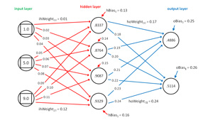
The neural network input-process-output computations are implemented in class function computeoutputs. The mechanism is illustrated in Figure 2. To keep the size of the figure small and the ideas clear, the neural network in the figure does not correspond to the demo neural network. The network in the figure has three input nodes, four hidden nodes, and two output nodes.
 [Click on image for larger view.]
Figure 2. Computing Neural Network Output Values
[Click on image for larger view.]
Figure 2. Computing Neural Network Output Values
The input values are {1.0, 5.0, 9.0}. The input-to-hidden weights are { 0.01, 0.02, . . 0.12 } and so on. The top-most hidden node value is 0.8337, which is computed as:
sum = (1.0)(0.01) + (5.0)(0.05) + (9.0)(0.09) + 0.13
    = 0.01 + 0.25 + 0.81 + 0.13
    = 1.20

value  = tanh(1.20)
       = 0.8337 (rounded)
The two pre-activation output node values are computed as:
output[0] sum = (.8337)(.17) + (.8764)(.19) + (.9087)(.21) + (.9329)(.23) + .25
              = 0.9636

output[1] sum = (.8337)(.18) + (.8764)(.20) + (.9087)(.22) + (.9329)(.24) + .26
              = 1.0091

output[0] value = softmax(0.9636, (0.9636, 1.0091))
                = e^0.9636 / (e^0.9636 + e^1.0091)
                = 2.6211 / (2.6211 + 2.7431)
                = 0.4886

output[1] value = softmax(1.0091, (0.9636, 1.0091))
                = e^1.0091 / (e^0.9636 + e^1.0091)
                = 2.7431 / (2.6211 + 2.7431)
                = 0.5114
Because softmax output values sum to 1.0, if the two dependent categorical variables in this dummy example were 1-of-N encoded as (1, 0) and (0, 1), because the second output node value is greater than the first, the computed output would be interpreted as the categorical value corresponding to (0, 1).
The Python code for function computeoutputs begins:
def computeoutputs(self, xValues):
  hSums = [0 for i in range(self.numHidden)]
  oSums = [0 for i in range(self.numOutput)]

  for i in range(len(xValues)):
    self.inputs[i] = xValues[i]
...
Here, lists for the pre-activation sums are initialized, and then the input values are copied from the xValues parameter (the training data) into the class inputs list. Next, the hidden node values are computed as described earlier:
for j in range(self.numHidden):
  for i in range(self.numInput):
    hSums[j] += (self.inputs[i] * self.ihWeights[i][j])

for i in range(self.numHidden):
  hSums[i] += self.hBiases[i]

for i in range(self.numHidden):
  self.hOutputs[i] = self.hypertan(hSums[i])
Next, the output node values are computed:
for j in range(self.numOutput):
  for i in range(self.numHidden):
    oSums[j] += (self.hOutputs[i] * self.hoWeights[i][j])

for i in range(self.numOutput):
  oSums[i] += self.oBiases[i]

softOut = self.softmax(oSums)
for i in range(self.numOutput):
  self.outputs[i] = softOut[i]
Function computeoutputs finishes by copying the computed node values into a local list and returning that list:
...
  result = [0 for i in range(self.numOutput)]
  for i in range(self.numOutput):
    result[i] = self.outputs[i]
  return result
Training the Neural Network
Neural network training is the process of finding the best values for the weights and biases so that when presented with the training data (which has known output values), the computed output values are very close to the known output values. Training a neural network is quite difficult. Among my colleagues, the three most common techniques for training a neural network are the back-propagation algorithm, simplex optimization and particle swarm optimization, with back-propagation being by far the most common of the three.
Because training is a fairly complex topic that needs an entire article itself, the example program uses a very rudimentary approach for demonstration purposes only. The basic idea is to just repeatedly guess random weights and bias values, keeping track of the set of values that gives the most accurate output values. The function definition begins:
def weaktrain(self, trainData, maxEpochs):
  # randomly guess weights
  numWts = ((self.numInput * self.numHidden) + self.numHidden +
    (self.numHidden * self.numOutput) + self.numOutput)
  bestAcc = 0.0
  bestWeights = [0 for i in range(numWts)]
  currAcc = 0.0
  currWeights = [0 for i in range(numWts)]
...
Variable bestAcc holds the best accuracy found. List bestWeights holds the weights and bias values that gave the best accuracy. Variable and list currAcc and currWeights are the current accuracy and weights and biases, respectively.
The main training loop is shown in Listing 4.
Listing 4: The Main Training Loop
lo = -10.0
hi = 10.0
epoch = 0
while epoch < maxEpochs:
  for i in range(len(currWeights)):
    currWeights[i] = (hi - lo) * self.rnd.random() + lo
  self.setweights(currWeights)
  currAcc = self.accuracy(trainData)
  if currAcc > bestAcc:
    bestAcc = currAcc
    for i in range(len(currWeights)):
      bestWeights[i] = currWeights[i]
  epoch += 1
The loop iterates maxEpochs times. A random set of weights and bias values is generated, those values are inserted into the neural network using function setweights, and then the accuracy is computed and checked against the best accuracy found so far. Python doesn't have a "++" operator so "+= 1" is typically used instead.
The training function concludes:
...
  self.setweights(bestWeights)
  result = self.getweights()
  return result
Let me emphasize that this training approach is for demonstration purposes only, although random training can sometimes be useful to establish baseline results before training with a realistic algorithm.
About the Author
Dr. James McCaffrey directs the data science and research efforts at Quaetrix, a data analytics company located near Redmond, Washington. Before joining Quaetrix, James was a senior research engineer at Microsoft. James can be reached at [email protected].