Neural Network Lab
Multi-Swarm Optimization for Neural Networks Using C#
Multi-swarm optimization (MSO) is a powerful variation of particle swarm optimization. Understanding how MSO works and how to implement it can be a valuable addition to your developer toolkit.
Many machine learning (ML) systems require code that minimizes error. In the case of neural networks, training a network is the process of finding a set of values for the network's weights and biases so that the error between the known output values in some training data and the computed output values is minimized. Algorithms that minimize error are also called optimization algorithms.
There are roughly a dozen different optimization algorithms commonly used in machine learning. For example, back-propagation is often used to train simple neural networks, and something called L-BFGS is often used to train logistic regression classifiers. Multi-swarm optimization (MSO) is one of my go-to algorithms for ML training, in particular with deep neural networks.
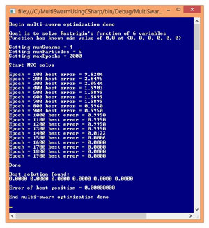
Take a look at the screenshot of a demo program in Figure 1. The demo uses MSO to solve a well-known benchmark problem called Rastrigin's function. Rastrigin's function can accept any number of input values; the number of inputs is called the dimension of the function. The demo uses Rastrigin's function with six dimensions. The minimum value of Rastrigin's function is 0.0 when all input values equal 0.
 [Click on image for larger view.]
Figure 1. Multi-Swarm Optimization in Action
[Click on image for larger view.]
Figure 1. Multi-Swarm Optimization in Action
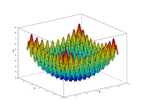
The graph in Figure 2 shows Rastrigin's function with two dimensions. The function has many hills and valleys that can trap optimization algorithms with an incorrect answer. The one global minimum value is at the bottom of the graph and isn't quite visible because of all the surrounding curves. Solving Rastrigin's function is quite difficult for optimization algorithms, which is why researchers often use it when investigating a new optimization algorithm.
 [Click on image for larger view.]
Figure 2. Rastrigin's Function for Two Variables
[Click on image for larger view.]
Figure 2. Rastrigin's Function for Two Variables
MSO is a variation of particle swarm optimization (PSO). In PSO, there are multiple virtual particles, where each particle represents a potential solution to the problem being solved. The collection of particles is called a swarm. The particles move, that is, change values, in a way that models the behavior of groups such as schools of fish and flocks of birds. MSO extends PSO by using several swarms that interact with each other.
The demo program uses four swarms. Each swarm has five particles. Larger numbers of swarms and particles increase the chance of finding the true minimum value, at the expense of slower performance. MSO is an iterative process. The demo sets a maximum number of iterations of the algorithm, in variable maxEpochs, to 2000. Again, more iterations is offset by slower performance.
Figure 1 shows the progress of the MSO algorithm every 100 epochs (iterations). In this case, MSO succeeded in finding the true minimum value of 0.0 at (0, 0, 0, 0, 0, 0). In realistic ML training scenarios, you won't know the true minimum error and usually have to employ some trial and error with the MSO parameters.
In this article, I'll explain how MSO works and walk you through the demo program. The code is a bit too long to present in its entirety, but the complete demo source code is available in the download that accompanies this article. I code the demo using C#, but you shouldn't have too much trouble refactoring the code to another language such as Visual Basic .NET or JavaScript.
Demo Program Structure
The overall structure of the demo program, with some minor edits to save space, is presented in Listing 1. All the control logic is contained in the Main method. Method Solve implements the MSO algorithm. Method Error accepts a particle's position (an array of type double), computes the value of Rastrigin's function at the position, and returns the absolute value of the difference between the computed value and the known minimum value of 0.0.
Class Particle encapsulates a particle's current position (a potential solution), current velocity (values used to update the particle's position), the error at the current position, the position of the best (smallest) error ever found by the particle, and the associated error at that best position.
Class Swarm is essentially an array of Particle objects, along with the best position found by any particle in the swarm, and the associated error of that best swarm position.
Listing 1: Overall Program Structure
using System;
namespace MultiSwarm
{
  class MultiSwarmProgram
  {
    static void Main(string[] args)
    {
      Console.WriteLine("Begin multi-swarm optimization demo");

      int dim = 6;
      Console.WriteLine("Goal is to solve Rastrigin's function of " +
        dim + " variables");
      Console.Write("Function has known min value of 0.0 at (");
      for (int i = 0; i < dim -1; ++i)
        Console.Write("0, ");
      Console.WriteLine("0)");

      int numSwarms = 4;
      int numParticles = 5;
      int maxEpochs = 2000;
      double minX = -10.0;
      double maxX = 10.0;

      Console.WriteLine("Start MSO solve");
      double[] bestPosition = Solve(dim, numSwarms,
        numParticles, maxEpochs, minX, maxX);
      double bestError = Error(bestPosition);
      Console.WriteLine("Done");

      Console.WriteLine("Best solution found: ");
      ShowVector(bestPosition, 4, true);
      Console.WriteLine("Error of best position = " +
        bestError.ToString("F8"));

      Console.WriteLine("End multi-swarm optimization demo");
      Console.ReadLine();
    } // Main

    static void ShowVector(double[] vector,
      int decimals, bool newLine) { . . }
    static double[] Solve(int dim, int numSwarms, int numParticles,
      int maxEpochs, double minX, double maxX) { . . }
    public static double Error(double[] position) { . . }
  }

  public class Particle
  {
    static Random ran = new Random(0);
    public double[] position;
    public double[] velocity;
    public double error;
    public double[] bestPartPosition;
    public double bestPartError;

    public Particle(int dim, double minX, double maxX) // random position
    {
      position = new double[dim];
      velocity = new double[dim];
      bestPartPosition = new double[dim];
      for (int i = 0; i < dim; ++i)
      {
        position[i] = (maxX - minX) * ran.NextDouble() + minX;
        velocity[i] = (maxX - minX) * ran.NextDouble() + minX;
      }
      error = MultiSwarmProgram.Error(position);
      bestPartError = error;
      Array.Copy(position, bestPartPosition, dim);
    }
  } // Particle

  public class Swarm
  {
    public Particle[] particles;
    public double[] bestSwarmPosition;
    public double bestSwarmError;

    public Swarm(int numParticles, int dim, double minX, double maxX)
    {
      bestSwarmError = double.MaxValue;
      bestSwarmPosition = new double[dim];
      particles = new Particle[numParticles];
      for (int i = 0; i < particles.Length; ++i)
      {
        particles[i] = new Particle(dim, minX, maxX); // random position
        if (particles[i].error < bestSwarmError)
        {
          bestSwarmError = particles[i].error;
          Array.Copy(particles[i].position, bestSwarmPosition, dim);
        }
      }
    }
  } // Swarm
} // ns
To create the demo program, I launched Visual Studio and created a C# console application named MultiSwarm. The demo has no significant .NET dependencies so any version of Visual Studio should work. After the template-generated code loaded into the Visual Studio editor, in the Solution Explorer window I renamed file Program.cs to the more descriptive MultiSwarmProgram.cs and Visual Studio automatically renamed class Program for me. At the top of the source code, I removed all unnecessary references to .NET namespaces, leaving just the reference to the top-level System namespace.
The key statements in the Main method are:
int dim = 6;
int numSwarms = 4;
int numParticles = 5;
int maxEpochs = 2000;
double minX = -10.0;
double maxX = 10.0;
double[] bestPosition = Solve(dim, numSwarms,
  numParticles, maxEpochs, minX, maxX);
double bestError = Error(bestPosition);
The purposes of variables dim, numSwarms, numParticles, and maxEpochs should be clear to you based on my earlier explanation of MSO. Variables minX and maxX establish upper and lower limits on the values in each component of a particle's position vector. Put another way, for Rastrigin's function of six variables, a particle's position will be an array with six cells, each of which holds a value between -10.0 and +10.0. These values are typical for ML systems where input data has been normalized in some way.
The Solve method returns the best position (location of the smallest error) found by any particle, in any swarm, during the MSO search process. That best position is passed to the Error method to get the associated error. An alternative design is to implement method Solve so that it returns the associated best error as an out-parameter.
The MSO Algorithm
In high-level pseudo-code, the MSO algorithm is presented in Listing 2. The key to the algorithm is how a particle's new velocity is calculated. In math terms the new velocity is:
v(t+1) = w * v(t) +
         (c1 * r1) * (p (t) - x(t)) +
         (c2 * r2) * (s (t) - x (t)) +
         (c3 * r3) * (g (t) - x (t))
After a new velocity has been computed, a particle's new position is:
x (t+1) = x (t) + v (t+1)
The term v(t+1) means the velocity at time t+1, in other words, the new velocity. Term v(t) is the current velocity. Term x (t) is the current position. Notice that x and v are in bold, which indicates they're vectors such as (8.0, -6.0) rather than single values.
Term p (t) is the position of the particle's best-known position. Term s (t) is the best position of any particle in the particle's swarm. Term g (t) is the global best position of any particle in any swarm.
Term w is a constant called the inertia factor. Terms c1, c2 and c3 are constants that establish a maximum change for each component of the new velocity. Terms r1, r2 and r3 and random values between 0 and 1 that provide a randomization effect to each velocity update.
The new velocity computation is probably best explained by example. Suppose a problem has dim set to 2 and a particle is currently at (20.0, 30.0) and its current velocity is (-1.0, -3.0). Also, the best-known position of the particle is (10.0, 12.0), the best-known position of any particle in the swarm is (8.0, 9.0), and the best-known position of any particle in any swarm is (5.0, 6.0). And suppose that constant w has value 0.7, constants c1 and c2 are both 1.4, and constant c3 is 0.4. Finally, suppose random values r1, r2 and r3 are all 0.2.
The new velocity of the particle (with rounding to one decimal) is:
v (t+1) = 0.7 * (-1.0, -3.0) +
         (1.4 * 0.2) * ((10.0, 12.0) - (20.0, 30.0)) +
         (1.4 * 0.2) * ((8.0, 9.0) - (20.0, 30.0)) +
         (0.4 * 0.2) * ((5.0, 6.0) - (20.0, 30.0))

       = 0.7 * (-1.0, -3.0) +
         0.3 * (-10.0, -18.0) +
         0.3 * (-12.0, -21.0) +
         0.1 * (-15.0, -24.0)

       = (-0.7, -2.1) +
         (-3.0, -5.4) +
         (-3.6, -6.3) +
         (-1.5, -2.4)

       = (-8.8, -16.2)
And so the particle's new position is:
x (t+1) = (20.0, 30.0) + (-8.8, -16.2)
       = (11.2, 13.8)
Assuming the optimal solution is at (0.0, 0.0), as is the case with Rastrigin's function, notice that the particle has moved from its original position (20.0, 30.0) to a new position (11.2, 13.8) that's much closer to the optimal solution.
The inertia term, w, in v (t+1) encourages a particle to continue moving in its current direction. The p (t) term encourages a particle to move toward its historical best-known position. The s (t) term encourages a particle to move toward the best-known position found by any of the particle's swarm-mates. The g (t) term encourages a particle to move toward the best-known position found by any particle in any swarm.
Constants c1, c2, and c3 are sometimes called the cognitive, social, and global weights. Those constants, along with random values r1, r2 and r3, and the inertia weight, determine how much each term influences the motion of a particle. Some research in regular PSO suggests reasonable values for w, c1 and c2 are 0.729, 1.49445 and 1.49445, respectively. There's little research on the c3 constant in MSO, but I typically use 0.3645 (half of the inertia weight), which has worked well for me in practice.
Listing 2: Multi-Swarm Algorithm Pseudo-Code
for-each swarm loop
  create particles at random positions
end for

while epoch < maxEpochs loop
  for-each swarm loop
    for-each particle in swarm loop

      does particle die?
      does particle immigrate?

      compute new velocity based on
        curr velocity, best particle position,
        best swarm position, and
        best overall position
      use new velocity to update position
      check if new position is a new particle
        best, or a new swarm best, or a new
        global best
    end each swarm
  end each particle
end while
return best global position found
In the pseudo-code in Listing 2, notice that before a particle moves, it may die (and be replaced by a new particle at a random position), or it may immigrate (swap swarms with a randomly selected particle). The death and immigration mechanisms add an element of randomness to MSO and help prevent the algorithm from getting stuck at a non-optimal solution.
Implementing the Solve Method
The definition of method Solve begins:
static double[] Solve(int dim, int numSwarms, int numParticles,
  int maxEpochs, double minX, double maxX)
{
  Random rnd = new Random(0);
  Swarm[] swarms = new Swarm[numSwarms];
  for (int i = 0; i < numSwarms; ++i)
    swarms[i] = new Swarm(numParticles, dim, minX, maxX);
  double[] bestMultiPosition = new double[dim];
  double bestMultiError = double.MaxValue;
...
Random object rnd is used by MSO in several places, as you'll see shortly. Here, the seed value is hardcoded as 0; you may want to pass the seed as a parameter to Solve. After allocating a Swarm object array of size numSwarms, each Swarm is instantiated by calling the Swarm constructor, which in turn calls the Particle constructor. The result is a collection of swarms, each with particles at random positions.
After the swarms are initialized, the swarms are examined to find the best error (smallest) and position of any of the particles in any of the swarms:
for (int i = 0; i < numSwarms; ++i)
{
  if (swarms[i].bestSwarmError < bestMultiError)
  {
    bestMultiError = swarms[i].bestSwarmError;
    Array.Copy(swarms[i].bestSwarmPosition, bestMultiPosition, dim);
  }
}
Next, the main MSO processing loop is prepared:
int epoch = 0;
double w = 0.729; // inertia
double c1 = 1.49445; // particle-cognitive
double c2 = 1.49445; // swarm-social
double c3 = 0.3645; // multiswarm-global
double pDeath = 0.005;      // prob of particle death
double pImmigrate = 0.005;  // prob of particle immigration
Notice the probabilities of death and immigration are fixed. An alternative is to make these values a function of the maximum number of loop iterations, for example, pDeath = maxEpochs / 5.0.
The main MSO processing loop begins:
while (epoch < maxEpochs)
{
  ++epoch;

  if (epoch % 100 == 0 && epoch < maxEpochs)
  {
    Console.WriteLine("Epoch = " + epoch + " best error = " +
      bestMultiError.ToString("F4"));
  }
. . .
Machine learning algorithms often require quite a bit of experimentation. Here, progress is displayed every 100 epochs. You might want to consider passing a Boolean "verbose" parameter to method Solve to control whether progress messages are displayed.
Next, each particle is examined, as shown in Listing 3.
Listing 3: Examining Each Particle
for (int i = 0; i < numSwarms; ++i) // Each swarm
{
  for (int j = 0; j < numParticles; ++j) // Each particle
  {
    double p1 = rnd.NextDouble();
    if (p1 < pDeath)
    {
      swarms[i].particles[j] = new Particle(dim, minX, maxX);
      if (swarms[i].particles[j].error < swarms[i].bestSwarmError)
      {
        swarms[i].bestSwarmError = swarms[i].particles[j].error;
        Array.Copy(swarms[i].particles[j].position, swarms[i].bestSwarmPosition, dim);
        if (swarms[i].particles[j].error < bestMultiError)
        {
          bestMultiError = swarms[i].particles[j].error;
          Array.Copy(swarms[i].particles[j].position, bestMultiPosition, dim);
        }
      }
    }
If a random value p1 is below the death threshold, the current particle is killed by calling the Particle constructor. The newly created particle must be checked to see if it is, by pure luck, at a new best position for its swarm or is a global best.
Next, the current particle may move to a different swarm, as shown in Listing 4.
Listing 4: Current Particle Moving to Different Swarm
double p2 = rnd.NextDouble();
if (p2 < pImmigrate)
{
  int otherSwarm = rnd.Next(0, numSwarms);
  int otherParticle = rnd.Next(0, numParticles);
  Particle tmp = swarms[i].particles[j];
  swarms[i].particles[j] = swarms[otherSwarm].particles[otherParticle];
  swarms[otherSwarm].particles[otherParticle] = tmp;
  if (swarms[i].particles[j].error < swarms[otherSwarm].bestSwarmError)
  {
    swarms[otherSwarm].bestSwarmError = swarms[i].particles[j].error;
    Array.Copy(swarms[i].particles[j].position,
      swarms[otherSwarm].bestSwarmPosition, dim);
  }
  if (swarms[otherSwarm].particles[otherParticle].error <
    swarms[i].bestSwarmError)
  {
    swarms[i].bestSwarmError =
      swarms[otherSwarm].particles[otherParticle].error;
    Array.Copy(swarms[otherSwarm].particles[otherParticle].position,
      swarms[i].bestSwarmPosition, dim);
  }
}
If immigration is triggered, Solve picks a random particle within a random swarm, to swap with the current particle. Note that there's no guarantee the random swarm will be different from the current swarm. You might want to modify the code to ensure that immigration occurs between different swarms.
Next, the new velocity for the current particle is calculated, as described earlier (see Listing 5).
Listing 5: New Velocity Calculated for Current Particle
for (int k = 0; k < dim; ++k)
{
  double r1 = rnd.NextDouble();
  double r2 = rnd.NextDouble();
  double r3 = rnd.NextDouble();

  swarms[i].particles[j].velocity[k] =
    (w * swarms[i].particles[j].velocity[k]) +
    (c1 * r1 * (swarms[i].particles[j].bestPartPosition[k] -
    swarms[i].particles[j].position[k])) +
    (c2 * r2 * (swarms[i].bestSwarmPosition[k] -
    swarms[i].particles[j].position[k])) +
    (c3 * r3 * (bestMultiPosition[k] -
    swarms[i].particles[j].position[k]));

  if (swarms[i].particles[j].velocity[k] < minX)
    swarms[i].particles[j].velocity[k] = minX;
  else if (swarms[i].particles[j].velocity[k] > maxX)
    swarms[i].particles[j].velocity[k] = maxX;
}
After the new velocity is calculated, its component values are checked to make sure they're not too large in magnitude, to prevent the algorithm from moving particles too far in any one iteration. The velocity-limiting values of minX and maxX are arbitrary, but have worked well for me in practice.
After a new velocity is calculated, that velocity is used to move the current particle:
for (int k = 0; k < dim; ++k)
{
  swarms[i].particles[j].position[k] +=
    swarms[i].particles[j].velocity[k];

  if (swarms[i].particles[j].position[k] < minX)
    swarms[i].particles[j].position[k] = minX;
  else if (swarms[i].particles[j].position[k] > maxX)
    swarms[i].particles[j].position[k] = maxX;
}
The components of the current particle's new position are constrained; if any component is out-of-range, it is set to either minX or maxX. This approach has given me better results than the seemingly more logical alternative of setting an out-of-range component to a random value between minX and maxX.
Next, the error associated with the new particle position is determined and checked to see if it's a new best error for the current particle:
swarms[i].particles[j].error =
  MultiSwarmProgram.Error(swarms[i].particles[j].position);

if (swarms[i].particles[j].error <
  swarms[i].particles[j].bestPartError)
{
  swarms[i].particles[j].bestPartError =
    swarms[i].particles[j].error;
  Array.Copy(swarms[i].particles[j].position,
    swarms[i].particles[j].bestPartPosition, dim);
}
Next, the new position is checked to see if it is a new swarm-best or a new global-best, as shown in Listing 6.
Listing 6: Checking New Position
if (swarms[i].particles[j].error <
  swarms[i].bestSwarmError)
{
  swarms[i].bestSwarmError = swarms[i].particles[j].error;
  Array.Copy(swarms[i].particles[j].position,
    swarms[i].bestSwarmPosition, dim);
}

if (swarms[i].particles[j].error < bestMultiError)
{
  bestMultiError = swarms[i].particles[j].error;
  Array.Copy(swarms[i].particles[j].position,
    bestMultiPosition, dim);
}
As implemented, a new position cannot be a new global-best position if it's not also a swarm-best position, so the branching logic in Listing 6 could be shortened. However, the price for an extra if-then check is relatively small and allows easier modification of the algorithm logic later.
Method Solve finished by returning the best position found:
      } // each particle
    } // each swarm
  } // while
  return bestMultiPosition;
} // Solve
Here, a reference to array bestMultiPosition is returned. A slightly more robust approach would be to copy the values in bestMultiPosition to a local array, and then return a reference to that array.
Wrapping Up
The code and explanation presented in this article should give you a solid foundation for understanding and experimenting with multi-swarm optimization. MSO is really more of a meta-heuristic than an algorithm. By that I mean MSO is more of a set of guidelines, with much room for alternative approaches, instead of a rigid prescription.
MSO is moderately complex compared to other numeric optimization approaches such as simplex optimization. However, for some tasks, training deep neural networks in particular, MSO has been very effective for me. I'll demonstrate the use of MSO for deep neural network training next time.