Neural Network Lab
How To Use Resilient Back Propagation To Train Neural Networks
It's more complex than back propagation, but Rprop has advantages in training speed and efficiency.
Resilient back propagation (Rprop), an algorithm that can be used to train a neural network, is similar to the more common (regular) back-propagation. But it has two main advantages over back propagation: First, training with Rprop is often faster than training with back propagation. Second, Rprop doesn't require you to specify any free parameter values, as opposed to back propagation which needs values for the learning rate (and usually an optional momentum term). The main disadvantage of Rprop is that it's a more complex algorithm to implement than back propagation.
Think of a neural network as a complex mathematical function that accepts numeric inputs and generates numeric outputs. The values of the outputs are determined by the input values, the number of so-called hidden processing nodes, the hidden and output layer activation functions, and a set of weights and bias values. A fully connected neural network with m inputs, h hidden nodes, and n outputs has (m * h) + h + (h * n) + n weights and biases. For example, a neural network with 4 inputs, 5 hidden nodes, and 3 outputs has (4 * 5) + 5 + (5 * 3) + 3 = 43 weights and biases.
Training a neural network is the process of finding values for the weights and biases so that, for a set of training data with known input and output values, the computed outputs of the network closely match the known outputs. The most common technique used to train neural networks is the back-propagation algorithm. Back propagation requires a value for a parameter called the learning rate. The effectiveness of back propagation is highly sensitive to the value of the learning rate. Rprop was developed by researchers in 1993 in an attempt to improve upon the back-propagation algorithm.
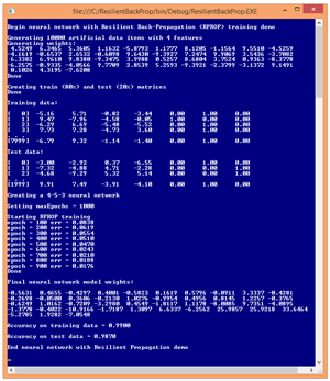
A good way to get a feel for what Rprop is, and to see where this article is headed, is to take a look at Figure 1. Instead of using real data, the demo program begins by creating 10,000 synthetic data items. Each data item has four features (predictor variables). The dependent Y value to predict can take on one of three possible categorical values. These Y values are encoded using 1-of-N encoding so Y can be (1, 0, 0) or (0, 1, 0), or (0, 0, 1).
 [Click on image for larger view.]
Figure 1. The Rprop Training Algorithm in Action
[Click on image for larger view.]
Figure 1. The Rprop Training Algorithm in Action
After generating the synthetic data, the demo randomly split the data set into an 8,000-item set to be used to train a neural network using Rprop, and a 2,000-item test set to be used to estimate the accuracy of the resulting model. The first training item is:
-5.16 5.71 -0.82 -3.44 0.00 1.00 0.00
All four feature values are between -10.0 and +10.0. You can imagine that the data corresponds to the problem of predicting which of three political parties (Republican, Democrat, Independent) a person is affiliated with, based on their annual income, age, socio-economic status, and education level, where the feature values have been normalized. So the first line of data could correspond to a person who has lower than average income (-5.16), and who is older than average (age = 5.71), with slightly lower than average socio-economic status (-0.82), and lower than average education level (-3.44), who is a Democrat (0, 1, 0).
The Rprop algorithm is an iterative process. The demo set the maximum number of iterations (often called epochs) to 1,000. As training progressed, the demo computed and displayed the current error, based on the best weights and biases found at that point, every 100 epochs. When finished training, the best values found for the 43 weights and biases were displayed. Using the best weights and bias values, the resulting neural network model had a predictive accuracy of 98.70 percent on the test data set.
This article assumes you have at least intermediate-level developer skills and a basic understanding of neural networks, but does not assume you know anything about the Rprop algorithm. The demo program is coded in C#, but you shouldn't have too much trouble refactoring the demo code to another language.
Understanding Gradients and the Rprop Algorithm
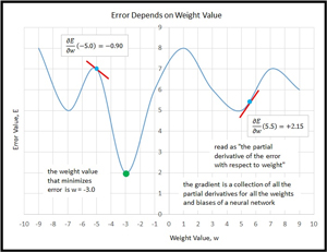
Many machine learning algorithms, including Rprop, are based on a mathematical concept called the gradient. I think using a picture is the best way to explain what a gradient is. Take a look at the graph in Figure 2. The curve plots error vs. the value of a single weight. The idea here is that you must have some measure of error (there are several), and that the value of the error will change as the value of one weight changes, assuming you hold the values of the other weights and biases the same. For a neural network with many weights and biases, there'd be graphs like the one in Figure 2 for every weight and bias.
 [Click on image for larger view.]
Figure 2. Partial Derivatives and the Gradient
[Click on image for larger view.]
Figure 2. Partial Derivatives and the Gradient
A gradient is made up of several "partial derivatives." A partial derivative for a weight can be thought of as the slope of the tangent line (the slope, not the tangent line itself) to the error function for some value of the weight. For example, in the figure, the "partial derivative of error with respect to weight" at weight = -5.0 is -0.90. The sign of the slope/partial derivative indicates which direction to go in order to get to a smaller error. A negative slope means go in the positive weight direction, and vice versa. The steepness (magnitude) of the slope indicates how rapidly the error is changing and gives a hint at how far to move to get to a smaller error.
Partial derivatives are called partial because they only take one weight into account; the other weights are assumed to be constant. A gradient is just a collection of the all-partial derivatives for all the weights and biases. Note that although the word gradient is singular, it has several components. Also, the terms gradient and partial derivative (or just "the partial," for brevity) are often used interchangeably when the meaning is clear from the context.
During training, regular back propagation uses the magnitudes of the partial derivatives to determine how much to adjust a weight value. This seems very reasonable, but if you look at Figure 2 you can see a drawback to this approach. Suppose a weight has a current value of -5.0 and regular back propagation sees a fairly steep gradient and calculates a weight delta of +7.0. The new weight value will be -5.0 + 7.0 = 2.0 and so the weight has gone well past the optimum value at -3.0. On the next iteration of training, the weight could swing wildly back and overshoot again but in the other direction. This oscillation could continue and the weight for the minimum error would never be found.
With regular back propagation, you normally use a small learning rate, which, along with the magnitude of the gradient, determines the weight delta in a training iteration. This means you likely won't overshoot an optimal answer, but it means training will be very slow as you creep closer and closer to a weight that gives minimum error.
The Rprop algorithm makes two significant changes to the back-propagation algorithm. First, Rprop doesn't use the magnitude of the gradient to determine a weight delta; instead, it uses only the sign of the gradient. Second, instead of using a single learning rate for all weights and biases, Rprop maintains separate weight deltas for each weight and bias, and adapts these deltas during training.
The original version of the Rprop algorithm was published in a 1993 paper, "A Direct Adaptive Method for Faster Back Propagation Learning: The Rprop Algorithm," by M. Riedmiller and H. Braun (PDF here). Several variations of Rprop have been published since the original paper. The demo program follows the original version of the algorithm closely, however, the descriptions of some parts of the algorithm are ambiguous and can be interpreted in more than one way.
In very high-level pseudo-code, the Rprop algorithm is presented in Listing 1. If you refer to Figure 2, you'll see that for a particular weight or bias, if the previous and current partial derivatives have the same sign, then that means the weight value hasn't skipped past the value that gives a minimum error, so you want to keep moving in the same direction. In fact, you can move faster so you increase the amount you added on the last iteration.
Listing 1: The Rprop Algorithm
while epoch < maxEpochs loop
  calculate gradient over all training items
  for each weight (and bias) loop
    if prev and curr partials have same sign
      increase the previously used delta
      update weight using  new delta
    else if prev and curr partials have different signs
      decrease the previously used delta
      revert weight to prev value
    end if
    prev delta = new delta
    prev gradient = curr gradient
  end-for
  ++epoch
end-while
return curr weights and bias values
But if the signs of the previous and current partials have changed, you've gone too far. So you move back to where you were in the previous iteration, and decrease the amount you added on the last iteration, so you won't move so far next time. The Rprop algorithm itself is quite simple, beautiful and elegant, but implementing it is not trivial because there are many hidden details.
The Demo Program
To create the demo program, I launched Visual Studio, selected the C# console application program template, and named the project ResilientBackProp. The demo has no significant Microsoft .NET Framework version dependencies so any relatively recent version of Visual Studio should work. After the template code loaded, in the Solution Explorer window I renamed file Program.cs to RpropProgram.cs and Visual Studio automatically renamed class Program for me.
The demo program is too long to present in its entirety in this article, but the entire source code is available in the accompanying file download. All normal error checking was been removed to keep the main ideas as clear as possible.
The overall structure of the demo program is presented in Listing 2. I removed unneeded using statements that were generated by the Visual Studio console application template, leaving just the one referencing the top-level System namespace.
Listing 2: Demo Program Structure
using System;
namespace ResilientBackProp
{
  class RpropProgram
  {
    static void Main(string[] args)
    {
      Console.WriteLine("Begin demo");
      . . .
      Console.WriteLine("End demo");
      Console.ReadLine();
    } // Main

    static double[][] MakeAllData(int numInput, int numHidden,
      int numOutput, int numRows, int seed) { . . }

    static void MakeTrainTest(double[][] allData,
      double trainPct, int seed,
      out double[][] trainData, out double[][] testData) { . . }

    public static void ShowData(double[][] data, int numRows,
      int decimals, bool indices) { . . }

    public static void ShowVector(double[] vector, int decimals,
      int lineLen, bool newLine)
  } // Program class

  public class NeuralNetwork
  {
    private int numInput;
    private int numHidden;
    private int numOutput;

    private double[] inputs;
    private double[][] ihWeights;
    private double[] hBiases;
    private double[] hOutputs;

    private double[][] hoWeights;
    private double[] oBiases;
    private double[] outputs;

    private Random rnd;

    public NeuralNetwork(int numInput, int numHidden,
      int numOutput) { . . }

    private static double[][] MakeMatrix(int rows,
      int cols, double v) { . . }

    private static double[] MakeVector(int len,
      double v) { . . }

    private void InitializeWeights() { . . }

    public double[] TrainRPROP(double[][] trainData,
      int maxEpochs) { . . }

    private static void ZeroOut(double[][] matrix) { . . }
    private static void ZeroOut(double[] array) { . . }

    public void SetWeights(double[] weights) { . . }
    public double[] GetWeights() { . . }

    public double[] ComputeOutputs(double[] xValues) { . . }
    private static double HyperTan(double x) { . . }
    private static double[] Softmax(double[] oSums) { . . }

    public double Accuracy(double[][] testData,
      double[] weights) { . . }
    private static int MaxIndex(double[] vector) { . . }

    public double MeanSquaredError(double[][] trainData,
      double[] weights) { . . }
  } // NeuralNetwork class
} // ns
All the control logic is in the Main method and all the classification logic is in a program defined NeuralNetwork class. Helper method MakeAllData generates a synthetic data set. Method MakeTrainTest splits the synthetic data into training and test sets. Methods ShowData and ShowVector are used to display training and test data, and neural network weights.
The Main method (with a few minor edits to save space) begins by preparing to create the synthetic data:
static void Main(string[] args)
{
  Console.WriteLine("Begin RPROP demo");
  int numInput = 4; // Number features
  int numHidden = 5; // Arbitrary
  int numOutput = 3; // Classes for Y
  int numRows = 10000;
  int seed = 0;
...
Next, the synthetic data is created:
  Console.WriteLine("Generating " + numRows +
    " artificial data items with " + numInput + " features");
  double[][] allData = MakeAllData(numInput, numHidden, numOutput,
    numRows, seed);
  Console.WriteLine("Done");
...
To create the 10,000-item synthetic data set I use helper method MakeAllData. That method creates a local neural network with random weights and bias values. Then, for each of the data items, random input values are generated, the output is computed by the local neural network using the random weights and bias values, and then output is converted to 1-of-N format.
Next, the demo program splits the synthetic data into training and test sets using these statements:
Console.WriteLine("Creating train and test matrices");
double[][] trainData;
double[][] testData;
MakeTrainTest(allData, 0.80, seed,
 out trainData, out testData);
Console.WriteLine("Done");
Console.WriteLine("Training data: ");
ShowData(trainData, 4, 2, true);
Console.WriteLine("Test data: ");
ShowData(testData, 3, 2, true);
Next, the neural network is instantiated like so:
Console.WriteLine("Creating a 4-5-3 neural network");
NeuralNetwork nn = new NeuralNetwork(numInput, numHidden, numOutput);
The neural network has four inputs (one for each feature) and three outputs (because the Y variable can be one of three categorical values. The choice of five hidden processing units for the neural network is the same as the number of hidden units used to generate the synthetic data, but in general, finding a good number of hidden units requires trial and error. Next, the Rprop training is accomplished with these statements:
int maxEpochs = 1000;
Console.WriteLine("Setting maxEpochs = " + maxEpochs);
Console.WriteLine("Starting RPROP training");
double[] weights = nn.TrainRPROP(trainData, maxEpochs);
Console.WriteLine("Done");
Console.WriteLine("Final neural network model weights:");
ShowVector(weights, 4, 10, true);
The maximum number of epochs to use for training is another parameter that, in general, must be determined through trial and error. Here, using 1,000 iterations was arbitrary. Notice that calling the Rprop training method is very simple and that unlike regular back propagation there are no parameters such as a learning rate and a momentum term. The demo program concludes by calculating the prediction accuracy of the neural network model:
...
  double trainAcc = nn.Accuracy(trainData, weights);
  Console.WriteLine("Accuracy on training data = " +
    trainAcc.ToString("F4"));
  double testAcc = nn.Accuracy(testData, weights);
  Console.WriteLine("Accuracy on test data = " +
    testAcc.ToString("F4"));
  Console.WriteLine("End RPROP demo");
  Console.ReadLine();
} // Main
The accuracy of the model on the test data gives you a very rough estimate of how accurate the model will be when presented with new data that has unknown output values. The accuracy of the model on the training data is useful to determine if model over-fitting has occurred. If the prediction accuracy of the model on the training data is significantly greater than the accuracy on the test data, then there's a good chance model over-fitting has happened.
Implementing Rprop Training
The definition of the Rprop training method begins with:
public double[] TrainRPROP(double[][] trainData,
  int maxEpochs)
{
  double[] hGradTerms = new double[numHidden]; // intermediate values
  double[] oGradTerms = new double[numOutput]; // h = hidden, o = output
...
The most difficult part of understanding Rprop is that the algorithm needs to calculate and save lots of information. When calculating a gradient for a weight or bias, a term associated with each hidden and output node must be calculated. Local arrays hGradTerms and oGradTerms store these intermediate values.
Next, matrices and arrays to save the gradient values for each weight and bias are instantiated:
double[][] hoWeightGradsAcc = MakeMatrix(numHidden, numOutput, 0.0);
double[][] ihWeightGradsAcc = MakeMatrix(numInput, numHidden, 0.0);
double[] oBiasGradsAcc = new double[numOutput];
double[] hBiasGradsAcc = new double[numHidden];
For a neural network, the gradients for weights and biases associated with output nodes are calculated differently than the gradients for weights and biases associated with hidden nodes. Additionally, the Rprop algorithm accumulates gradient values for each weight and bias over all training items, so I append an "Acc" (for accumulated) to each name. Method MakeMatrix is just a helper to allocate and initialize an array-of-arrays-style matrix.
Next, matrices and arrays to store the gradient values for each weight and bias on the previous iteration of algorithm are instantiated:
double[][] hoPrevWeightGradsAcc = MakeMatrix(numHidden, numOutput, 0.0);
double[][] ihPrevWeightGradsAcc = MakeMatrix(numInput, numHidden, 0.0);
double[] oPrevBiasGradsAcc = new double[numOutput];
double[] hPrevBiasGradsAcc = new double[numHidden];
A key idea of the Rprop algorithm is that the delta amount to add to a weight or bias is different for each weight and bias, and depends on the amount added in the previous iteration. Matrices and arrays to store that information are set up like so:
double[][] hoPrevWeightDeltas = MakeMatrix(numHidden, numOutput, 0.01);
double[][] ihPrevWeightDeltas = MakeMatrix(numInput, numHidden, 0.01);
double[] oPrevBiasDeltas = MakeVector(numOutput, 0.01);
double[] hPrevBiasDeltas = MakeVector(numHidden, 0.01);
Next, some Rprop parameters are set up with this code:
double etaPlus = 1.2;
double etaMinus = 0.5;
double deltaMax = 50.0;
double deltaMin = 1.0E-6;
The numeric values come from the research paper that introduced the Rprop algorithm. Variable etaPlus is the factor used to increase a weight or bias delta when the algorithm is moving in the correct direction. Variable etaMinus is the factor used to decrease a weight or bias delta when the algorithm has overshot a minimum error. Variables deltaMax and deltaMin are used to prevent any weight or bias increase or decrease factor from being too large or too small.
The main processing loop begins with:
int epoch = 0;
while (epoch < maxEpochs)
{
  ++epoch;
  if (epoch % 100 == 0 && epoch != maxEpochs)
  {
    double[] currWts = this.GetWeights();
    double err = MeanSquaredError(trainData, currWts);
    Console.WriteLine("epoch = " + epoch +
      " err = " + err.ToString("F4"));
  }
...
Here, the current error is calculated and displayed every 100 epochs. This is an expensive operation, but useful to monitor training progress. You might want to consider passing a "verbose" parameter to method TrainRPROP to determine whether to display progress information.
The main loop starts by calculating accumulated gradients for each weight and bias. This isn't easy or quick. The first part of the code is:
ZeroOut(hoWeightGradsAcc);
ZeroOut(ihWeightGradsAcc);
ZeroOut(oBiasGradsAcc);
ZeroOut(hBiasGradsAcc);

double[] xValues = new double[numInput]; // Inputs
double[] tValues = new double[numOutput]; // Targets
Overloaded helper method ZeroOut assigns 0.0 to the accumulated gradient values from the previous iteration. Local arrays xValues and tValues are used to hold the input and target/desired output values from the current training item.
The loop to walk through all training items to accumulate gradient values begins by computing intermediate gradient values for the hidden-to-output weights and biases, like so:
for (int row = 0; row < trainData.Length; ++row)
{
  Array.Copy(trainData[row], xValues, numInput);
  Array.Copy(trainData[row], numInput, tValues, 0, numOutput);
  ComputeOutputs(xValues);
  for (int i = 0; i < numOutput; ++i)
  {
    double derivative = (1 - outputs[i]) * outputs[i];
    oGradTerms[i] = derivative * (outputs[i] - tValues[i]);
  }
Conceptually, there is a lot going on here. The first three statements fetch the input and target values from the current training item, and then compute and store the output values. To calculate the gradient associated with a node, you need the calculus derivative of the activation function used for the node. Here, the neural network uses the softmax function, which, if output is O and target value is T, has a derivative of (1 - O) * O. The gradient term for the node (but not the actual gradient of the associated weight or bias) is (1 - O) * O * (O - T). Yes, this is extremely deep information and not at all obvious even if you're fairly experienced with neural networks.
Next, the gradient terms of the input-to-hidden weights and biases are calculated:
for (int i = 0; i < numHidden; ++i)
{
  double derivative = (1 - hOutputs[i]) * (1 + hOutputs[i]);
  double sum = 0.0;
  for (int j = 0; j < numOutput; ++j)
  {
    double x = oGradTerms[j] * hoWeights[i][j];
    sum += x;
  }
  hGradTerms[i] = derivative * sum;
}
The neural network uses the hyperbolic tangent function, often abbreviated tanh, for hidden node activation. The tanh function has a derivative of (1 - O) * (1 + O). Notice the input-to-hidden gradient terms require the hidden-to-output gradient terms. This is why back propagation is named as it is (the calculations must move backward, from output to input).
Next, the intermediate output gradient terms are combined with their associated inputs to calculate and accumulate the gradients for the hidden-to-output weights:
for (int i = 0; i < numHidden; ++i)
{
  for (int j = 0; j < numOutput; ++j)
  {
    double grad = oGradTerms[j] * hOutputs[i];
    hoWeightGradsAcc[i][j] += grad;
  }
}
Next, the output node bias gradients are calculated and accumulated:
for (int i = 0; i < numOutput; ++i)
{
  double grad = oGradTerms[i] * 1.0; // Dummy input
  oBiasGradsAcc[i] += grad;
}
Biases can be thought of as weights that have a constant 1.0 associated input. Here, I explicitly use that dummy input but in most cases you'd want to leave out the unnecessary multiplication.
Next, the input-to-hidden weight gradients are calculated and accumulated:
for (int i = 0; i < numInput; ++i)
{
  for (int j = 0; j < numHidden; ++j)
  {
    double grad = hGradTerms[j] * inputs[i];
    ihWeightGradsAcc[i][j] += grad;
  }
}
At about this point you might get the feeling that code like this is overwhelming, but trust me, if you examine it enough times, each part of the puzzle eventually becomes understandable. Next, the hidden bias gradients are calculated and accumulated, which completes the process of calculating accumulated gradients for all weights and biases:
...
  for (int i = 0; i < numHidden; ++i)
  {
    double grad = hGradTerms[i] * 1.0;
    hBiasGradsAcc[i] += grad;
  }
} // Each row of training data
After all gradients have been calculated, the heart of the Rprop algorithm starts. Unlike gradients, which must be calculated from output back to input, the weights and biases can be updated in any order. Method TrainRPROP updates the input-to-hidden weights first. Listing 3 shows how that code begins.
Listing 3: Beginning Code for Updating Weights and Biases
double delta = 0.0;
for (int i = 0; i < numInput; ++i)
{
  for (int j = 0; j < numHidden; ++j)
  {
    if (ihPrevWeightGradsAcc[i][j] *
      ihWeightGradsAcc[i][j] > 0) // No sign change
    {
      delta = ihPrevWeightDeltas[i][j] * etaPlus;
      if (delta > deltaMax) delta = deltaMax;
      double tmp = -Math.Sign(ihWeightGradsAcc[i][j]) * delta;
      ihWeights[i][j] += tmp; // Update weights
    }
...
If the product of the previous gradient and the current gradient is positive, that means both values were either positive or negative, which means the sign of the gradient hasn't changed. This means the algorithm is moving in the correct direction, so the amount to adjust a weight can be increased, in order to move faster. The Math.Sign function is used to determine the correct direction to adjust the weight. Next comes:
...
else if (ihPrevWeightGradsAcc[i][j] *
  ihWeightGradsAcc[i][j] < 0) // Sign change
{
  delta = ihPrevWeightDeltas[i][j] * etaMinus;
  if (delta < deltaMin) delta = deltaMin;
  ihWeights[i][j] -= ihPrevWeightDeltas[i][j];
  ihWeightGradsAcc[i][j] = 0;
}
If the product of the previous and current gradients is negative, that means the sign of the gradient has changed, which means the algorithm has gone past an optimal weight value. The delta value is decreased and saved for the next iteration, but not used. The weight value is reverted to its value from the previous iteration. The curious statement that sets the value of the gradient of the current weight to 0 is really sort of a coding hack to force execution to fall through to the next if-then branch on the next iteration:
...
    else // Product of prev and curr grads is 0
    {
      delta = ihPrevWeightDeltas[i][j]; // No change to delta
      double tmp = -Math.Sign(ihWeightGradsAcc[i][j]) * delta;
      ihWeights[i][j] += tmp; // update
    }
    ihPrevWeightDeltas[i][j] = delta; // Save delta
    ihPrevWeightGradsAcc[i][j] = ihWeightGradsAcc[i][j];
  } // j
} // i
This branch will execute if, on the previous iteration, the algorithm overshot the optimal weight value and so decreased delta and reverted the weight to its previous value. In this case, the weight is updated using the new, smaller delta.
Method TrainRPROP concludes by updating the remaining weights and biases, and then returning the final values for all weights and biases:
...
    // Update hidden biases
    // Update hidden-to-output weights
    // Update output biases
  } // While (each epoch)
  double[] wts = this.GetWeights();
  return wts;
} // Train
The pattern to update the remaining weights and biases follows the same pattern as that used to update the input-to-hidden weights.
Wrapping Up
The resilient back-propagation algorithm is often a fast, effective, and robust technique for training a neural network. But in practice, I just don't see Rprop used very often, at least by my colleagues. My hunch is that even though the Rprop algorithm itself is quite simple, as you've seen in this article, implementation is difficult, mostly because of all the details of keeping track of lots of information. But the explanation and code presented here should enable you to get up and running with Rprop training for neural networks.