The Data Science Lab
Results Are in -- the Sign Test Using R
The R language can be used to perform a sign test, which is handy for comparing "before and after" data.
The Sign Test is most often used in situations where you have "before and after" data and you want to determine if there was an effect of some sort. The idea is best explained by example. Suppose you're working at a pharmaceutical company and want to know if a new weight-loss drug is effective. You get 10 volunteers to use your drug for several weeks. You look at the weights of your 10 subjects before and after the experiment. Suppose eight out of 10 of the subjects lost weight. Do you have solid statistical evidence to suggest that your drug worked?
Here's a second example. Suppose you have 20 Web server machines and you apply a software patch designed to improve performance. You measure response times before applying the patch and after applying the patch. What can you conclude if 12 servers showed better performance, three servers showed no change and five servers showed worse performance?
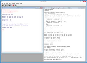
The best way to see where this article is headed is to take a look at the demo R session in Figure 1. In the sections that follow, I'll walk you through the demo script that generated the output. After reading this article, you'll have a solid grasp of what type of problem the Sign Test solves, know exactly how to perform a Sign Test using R, and understand how to interpret the results of a Sign Test. All of the source code for the demo program is presented in this article. You can also get the complete demo program in the code download that accompanies this article.
 [Click on image for larger view.]
Figure 1. Sign Test Using R
[Click on image for larger view.]
Figure 1. Sign Test Using R
In the R Console window, I entered an rm command to delete all objects from my current workspace. Then I entered a setwd command to point to the directory containing my demo script. And then I executed the demo using the source command. The demo program begins by setting up 10 pairs of before-after data points:
Begin Sign Test demo

Before:  80 90 95 85 70 80 85 60 70 85
After :  75 88 97 82 74 78 84 58 69 81
Here I'm imagining that the data correspond to a weight-loss (in kilograms) experiment, so when the after-value is smaller than the corresponding before-value, the data point is a "success." In the days before computers when the Sign Test was calculated manually, it was common to put a '+' sign next to successes and a '-' sign next to a failure. This is where the name of the Sign Test comes from. If you did add '+' and '-' signs, the raw data would look like:
Before:  80 90 95 85 70 80 85 60 70 85
After :  75 88 97 82 74 78 84 58 69 81
                     +    +     -     +     -     +    +     +    +     +
Next, the demo programs uses a function to count the number of successes and the number of failures, and displays those counts:
Num success =  8
Num failure =  2
Next, the demo uses the counts of successes and failures to perform a Sign Test, using the built-in R binom.test function, and then prints an interpretation message:
Executing binom.test
The prob of 'no effect' is  0.05692315
So the prob there was 'an effect' is  0.9430769

End Sign Test demo
The R language doesn't have a function named sign.test as you might have guessed there'd be. The mathematical Sign Test is actually a special case of the more general binominal test. And, as usual with R, it's up to you to interpret the output of an R function. For the Sign Test, you get a p-value, which is the probability of no effect. In this example, the probability of no effect is about 6 percent, which suggests that there is an effect. In other words, you have some statistical evidence that supports the notion that the weight-loss drug does work.
The Demo Program
If you want to copy-paste and run the demo program, and you don't have R installed on your machine, installation (and just as important, uninstallation) is quick and easy. Do an Internet search for "install R" and you'll find a URL to a page that has a link to "Download R for Windows." I'm using R version 3.3.0, but by the time you read this article, the current version of R will likely have changed. If you click on the download link, you'll launch a self-extracting executable installer program. You can accept all the installation option defaults, and R will install in about 30 seconds. Just as important, installing R will not hose your system, and you can quickly and cleanly uninstall R using the Windows Control Panel Programs and Features uninstall option.
To create the demo program, I navigated to directory C:\Program Files\R\R-3.3.0\bin\x64 and double-clicked on the Rgui.exe file. After the shell launched, from the menu bar I selected the File | New script option, which launched an untitled R Editor. I added two comments to the script, indicating the file name and R version I'm using:
# signTestDemo.R
# R 3.3.0
and then I did a File | Save as, to save the script. I put my demo script at C:\SignTestUsingR, but you can use any convenient directory.
The demo program begins by defining a function that accepts a before-vector and an after-vector, counts the number of successes and failures and "neithers," and returns those values in a vector with three cells. The definition of program-defined function signCounts begins with:
signCounts = function(before, after) {
  n <- length(before)
  result <- vector(mode="integer", length=3)
  # [1] = num neg (fail), [2] = num zero, [3] = num pos (success)
...
The function determines the length of both vectors just by using the before-vector parameter, so the assumption is that the before-vector and the after-vector have the same number of cells. The R language doesn't support out-parameters, so if you need to return more than one value, you can return a vector (or its cousin, a one-dimensional array).
The signCounts function has a comment that indicates where the count of failures (for this weight-loss example, when the after-value is greater than the before-value), the count of "neithers" (when the before-value equals the after value), and the count of successes are located. Unlike most languages, R vectors use one-based indexing rather than zero-based indexing.
The core code for function signCounts is:
for (i in 1:n) {
  if (before[i] - after[i] < 0) {
    result[1] <- result[1] + 1
  }
  else if (before[i] - after[i] > 0) {
    result[3] <- result[3] + 1
  }
  else {
    result[2] <- result[2] + 1
  }
}
The code counts successes, failures and "neithers" by subtracting each after-value from its corresponding before-value. This is a traditional approach in the Sign Test, but there's no reason not to simply compare each before-value and after-value directly, for example, if (before[i] < after[i]) { result[1] <- result[1] + 1 }.
Once you've worked a couple of examples, you'll find that the Sign Test is very simple. But you do have to be very careful to keep your definition of what a "success" is clear so you know exactly how to calculate successes and failures. Function signCounts concludes by returning the result-vector:
...
  return(result)
}
In R, return is a function rather than a keyword, so the parentheses are required syntax. The version of the signCounts function I've presented uses a standard loop-through-a-vector paradigm that can be used in most programming languages. But the R language has many high-level language abstractions that provide you with several alternative approaches. For example, function signCounts could have been coded as:
signCounts = function(before, after) {
  result <- vector(mode="integer", length=3)
  signedVals <- before - after
  result[1] <- sum(signedVals < 0)
  result[2] <- sum(signedVals = 0)
  result[3] <- sum(signedVals > 0)
  return(result)
}
Here, overloaded subtraction is applied to the before-vector and the after-vector parameters and the result is a vector that holds a cell-by-cell subtraction. And R has a strange idiom. The statement result[1] <- sum(signedVals < 0) will scan vector signedVals cell by cell, and count the number of cells that are negative.
Because I primarily work with C-family languages such as C# and JavaScript, I prefer using standard programming techniques rather than the many clever, but sometimes tricky, R language high-level programming abstractions. However, many of my colleagues prefer the short and sweet R programming tricks, especially when using R interactively.
The Main Part of the Program
After defining the helper function that counts successes and failures, the demo script sets up and displays the source data:
cat("\nBegin Sign Test demo \n\n")

before <- c(80, 90, 95, 85, 70, 80, 85, 60, 70, 85)
after  <- c(75, 88, 97, 82, 74, 78, 84, 58, 69, 81)

cat("Before: ", before, "\n")
cat("After : ", after, "\n\n")
Here the data is hardcoded and stored into two vectors using the tersely named c function. In many scenarios your source data will be in a text file. In those situations you can use the read.table function. For example, suppose you have a text file named BeforeAfter.txt that looks like:
BEFORE,AFTER
80,75
90,88
...
85,81
You could then write code like this:
mydf <- read.table("BeforeAfter.txt", header=TRUE, sep=",")
before <- mydf$BEFORE
after <- mydf$AFTER
These statements read the data in file BeforeAfter.txt into an R data frame object named mydf. Then the first column of the data frame is copied into a vector named before (using the '$' token), and the second column is copied into a vector named after.
After setting up the source data, the demo program calls the signCounts function like this:
sc <- signCounts(before, after)
numFail <- sc[1]
numZero <- sc[2]
numSucc <- sc[3]
Because there are only 10 pairs of data, you could have just visually scanned the data and determined the number of successes and failures manually, but a programmatic approach is preferable when you have a large data set. Next, the Sign Test is prepared with these statements:
N <- numFail + numSucc  # ignoring sign=0 cases
X <- numSucc

cat("Num success = ", numSucc, "\n")
cat("Num failure = ", numFail, "\n")
Here X holds the number of successes and N holds the total number of data points. In this example there are no data pairs where the before-value equals the after-value. But if there had been, those data points would've been ignored. This is the standard approach, but I'll have more to say about this topic shortly.
The actual Sign Test is performed by these statements:
cat("\nExecuting binom.test \n")
model <- binom.test(x=X, n=N, alternative="greater")  # 'exact'

cat("The prob of 'no effect' is ", model$p.value, "\n")
cat("So the prob there was 'an effect' is ", 1 - model$p.value, "\n")

cat("\nEnd Sign Test demo \n\n")
The results of the binom.test function are stored into an object named model. The binom.test function accepts the number of successes as parameter x, and the total number of data pairs as parameter n. The function also accepts a parameter named alternative, which is passed a value of "greater" in this example. The idea here is that for this weight-loss problem, an effect will have occurred when the number of successes (weight losses) is greater than what you'd get if there was no effect and weight losses and gains were just random.
The binom.test function also has a parameter named p that has a default value of 0.5. For the basic Sign Test, the value of p should be 0.5, so the demo program omits the explicit call to the p parameter.
The return result of the binom.test function is a list with nine named cells: statistic, parameter, p.value, estimate, null.value, conf.int, alternative, method and data.name. The most important result is the value in the p.value item, which is fetched by the demo program as model$p.value. The value of return result p.value for the demo data is 0.0569. Somewhat loosely, this represents the probability that there was no effect. Put differently, the p.value is the probability that you could see the observed number of successes if in fact the number of successes is random.
For this data, the probability that there is no effect is quite small, so you might say something like, "The p.value is 0.0569 so there is fairly strong statistical evidence that the observed data would not have occurred if there was no weight-loss effect." You should always interpret the results of statistical tests conservatively.
So, just how did I know that the return result had an item named p.value? In R you can either look up the documentation for a function, or you can type the command summary(model) to see details about the return result.
Two-Sided Tests and Approximate Tests
The example problem is called a one-sided, or one-tailed, test. Because you're looking at a weight-loss experiment, an effect is more weight losses (successes) than you'd get by chance. You can also perform a two-sided -- also called two-tailed -- Sign Test. For example, suppose you're doing an experiment with some sort of pain medication. As part of your experiment, you weigh your test subjects before and after the experiment. You'd have no reason to believe that the pain medication will affect weight. In other words, an effect would be either a weight loss or a weight gain.
To perform a two-sided Sign Test, all you have to do is change the call to the binom.test function:
model <- binom.test(x=X, n=N, alternative="two.sided")
The p.value for a two-sided binomial test will be exactly twice the p-value for a one-sided test. For the demo data, the p.value is 0.1094, and so the probability of no effect is greater.
The binom.test function calculates an exact p-value. In the days before computers, instead of calculating the exact p-value, which requires a lot of work, it was common to calculate an approximate p-value using some clever mathematics. The R language has a prop.test function that calculates an approximate p-value. For example:
model <- prop.test(x=X, n=N, alternative="greater")
For the demo data, the approximate p-value calculated by the prop.test function is 0.05692, which is very close to the exact value of 0.05692315. There's no real reason to use the prop.test in most situations.
Dealing with "Neithers" and the Curse of Symmetry
When working with paired before and after data, it's possible for the before-value to equal the after-value. In practice this is quite rare. The usual approach is to simply toss out (either manually or programmatically) those data items where the before-value equals the after-value. I don't agree with this approach. For one-sided tests, in my mind a no-change data item is conceptually a failure. However, for two-sided tests the situation isn't quite as clear and I decide to toss out neither-values on a case-by-case basis.
As you've seen in this article, the mechanics of the Sign Test using R are quite simple. The trickiest part of the Sign Test is keeping your definitions clear. There's potential confusion because there are multiple symmetries in every problem. You can define a success as an increase or decrease in an after-value. For example, in the weight-loss example, a success is a decrease in the after-value. But suppose your data represents test scores on some kind of exam before and after studying. A success would be an increase in the after-value. Additionally, if you're using manual + and - signs, either sign can represent a success or a failure. And the binom.test function can specify an alternative parameter of either "greater" or "less"
My approach when working with a Sign Test is to first define what I mean by a success. In one-sided scenarios (by far the most common in my work environment), I try to define a success as an expected result, as opposed to "something good." For example, if you were looking at cancer, an increase in a patient's cancer might be defined as a success. Then I write a custom function to count successes, failures and "neithers," where an after-value being greater than the corresponding before-value could mean a success or a failure, depending on the problem.
Wrapping Up
The Sign Test is an example of what's called a non-parametric statistical test. This means, in part, that the Sign Test doesn't make any assumptions about the distribution of the data being studied. Instead of using a Sign Test, it's possible to use what's called a paired t-test. For example, for the demo data you could enter these R commands:
pmodel <- t.test(before, after, paired=TRUE, alt="greater")
print(pmodel)
The result of this t-test is a p-value of 0.06615, which is quite close to the p-value of 0.05692 returned by the binom.test used for a Sign Test. However, the t-test is a parametric test. The t-test assumes that the population data has a normal (Gaussian, bell-shaped) distribution, which would be almost impossible to verify with a very small data set size. Because of this, when I want to investigate before and after data, I will usually use a Sign Test instead of a t-test.