The Data Science Lab
Neural Networks Using Python and NumPy
With Python and NumPy getting lots of exposure lately, I'll show how to use those tools to build a simple feed-forward neural network.
Over the past few months, the use of the Python programming language has increased greatly, at least among my colleagues who do data science and machine learning. I suspect this increase is due in large part to the release of two very powerful code libraries: Microsoft CNTK and Google TensorFlow. Both libraries have a Python API, which is the preferred interface.
Both libraries work at a fairly low level of abstraction, which means that a solid knowledge of Python is important when working with either library. Additionally, both libraries make extensive use of the "numerical Python" (NumPy) add-in package to create vectors and matrices, which typically offer better performance than Python's built-in list type.
In this article I'll explain how to implement a simple feed-forward neural network from scratch, using just Python 3.x and NumPy. After reading this article you should have a solid grasp of neural network fundamentals, as well as knowledge of Python and NumPy techniques that would be useful when working with CNTK or Tensorflow.
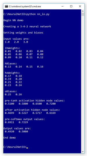
The best way to get a feel for where this article is headed is to take a look at the screenshot of a demo program shown in Figure 1. The demo Python program is designed to illustrate how the neural network input-output mechanism works. The demo does not create a prediction model as you'd do in a realistic scenario.
 [Click on image for larger view.]
Figure 1. Python Neural Network IO Demo
[Click on image for larger view.]
Figure 1. Python Neural Network IO Demo
The demo creates a neural network with three input nodes, four hidden processing nodes and two output nodes. If you're new to neural networks you can think of a neural network as a complex math function that accepts a set of numeric inputs and produces one or more numeric outputs.
The demo input values are (1.0, 2.0, 3.0) and the output values are (0.4920, 0.5080). The demo program displays the values of the neural net's so-called weights and bias values, which determine the output values for a given set of input values. The demo also displays some intermediate values (pre-activation hidden node values, and pre-activation output node values) that are calculated inside the neural net.
This article assumes you have a basic familiarity with Python or any C-family language such as C#, C/C++, JavaScript or Java, but does not assume you know anything about neural networks. The demo program is a bit too long to present in its entirety in this article, but the complete source code is available in the accompanying file download.
I wrote the demo using the 3.5 version of Python and the 1.11.1 version of NumPy. It is possible to install Python and NumPy separately; however, if you're new to Python and NumPy, I recommend installing the Anaconda distribution of Python, which simplifies installation and gives you many additional useful packages.
Understanding Neural Network Input-Output
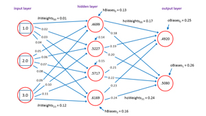
Before looking at the demo code, it's important to understand the neural network input-output mechanism. The diagram in Figure 2 corresponds to the demo program.
 [Click on image for larger view.]
Figure 2. Neural Network Input-Output
[Click on image for larger view.]
Figure 2. Neural Network Input-Output
The input node values are (1.0, 2.0, 3.0). Each blue line connecting input-to-hidden and hidden-to-output nodes represents a numeric constant called a weight. If nodes are zero-based indexed with node [0] at the top of the diagram, then the weight from input[0] to hidden[0] is 0.01, and the weight from hidden[3] to output[1] is 0.24.
Each hidden node and each output node (but not the input nodes) has an additional special weight called a bias. The bias value for hidden[3] is 0.16 and the bias for output[0] is 0.25.
Notice that if there are ni input nodes and nh hidden nodes and no output nodes. Then there are a total of (ni * nh) + (nh * no) + nh + no weights and biases. For the demo 3-4-2 neural net there are (3 * 4) + (4 * 2) + 4 + 2 = 26 weights and bias values.
In words, to compute the value of a hidden node, you multiply each input value times its associated input-to-hidden weight, add the products up, then add the bias value, and then apply the hyperbolic tangent function to the sum. For hidden[0] this is:
sum[0] = (1.0)(0.01) + (2.0)(0.05) + (3.0)(0.09) + 0.13
            = 0.5100

hidden[0] = tanh(0.5100)
                = 0.4699
The tanh function is called the neural network hidden layer activation function. The tanh function forces all hidden node values to be between -1.0 and +1.0. A common alternative activation function is the logistic sigmoid function.
The output nodes are calculated similarly, but instead of using tanh or logistic sigmoid activation, a special function called softmax is used for activation. The preliminary sum of products plus bias values of output[0] and output[1] are:
sum[0] = (0.4699)(0.17) + (0.5227)(0.19) + (0.5717)(0.21) + (0.6169)(0.23) + 0.25
            = 0.6911

sum[1] = (0.4699)(0.18) + (0.5227)(0.20) + (0.5717)(0.22) + (0.6169)(0.24) + 0.26
            = 0.7229
The softmax function is perhaps best explained by example:
divisor = exp(0.6911) +  exp(0.7229)
            = 1.9960 + 2.0604
            = 4.0563

output[0] = 1.9960 / 4.0563
               = 0.4920

ouput[1] = 2.0604 / 4.0563
              = 0.5080
Notice that softmax uses the exp(x) function, which can be astronomically large for even moderate values of x. The demo program uses a clever algebra trick ("the softmax max trick") to reduce the possibility of arithmetic overflow.
The purpose of softmax activation is to scale output values so that they sum to 1.0 and can be interpreted as probabilities. Suppose the demo corresponded to a problem where the goal is to predict if a person is male or female based on three predictor variables such as annual income, years of education and height. If male is encoded as (1, 0) and female is encode as (0, 1), then the prediction is female because the second output value (0.5080) is larger than the first (0.4920). Note: It's relatively uncommon to use (1, 0) and (0, 1) encoding for a binary classification problem, but I used this encoding in the explanation to match the demo neural network architecture.
Overall Program Structure
The overall program structure is presented in Listing 1. To edit the demo program I used the simple Notepad++ program. Most of my colleagues prefer using one of the many nice Python editors that are available.
I commented the name of the program and indicated the Python version used. I added three import statements to gain access to the NumPy package, and the math and random modules. As I mentioned earlier, the use of the NumPy package is becoming increasingly common.
Listing 1: Overall Program Structure
# nn_io.py
# Python 3.x

import numpy as np
import random
import math

# ------------------------------------

def showVector(v, dec): . . .
def showMatrix(m, dec): . . .

# ------------------------------------

class NeuralNetwork: . . .

# ------------------------------------

def main():
  print("\nBegin NN demo \n")

  # np.random.seed(0)  # does not affect the NN
  numInput = 3
  numHidden = 4
  numOutput = 2
  print("Creating a %d-%d-%d neural network " %
    (numInput, numHidden, numOutput) )
  nn = NeuralNetwork(numInput, numHidden, numOutput)

  print("\nSetting weights and biases ")
  numWts = NeuralNetwork.totalWeights(numInput, numHidden,
    numOutput)
  wts = np.zeros(shape=[numWts], dtype=np.float32)
  for i in range(len(wts)):
    wts[i] = ((i+1) * 0.01)  # [0.01, 0.02, . . . ]
  nn.setWeights(wts)

  # wts = nn.getWeights()  # verify weights
  # showVector(wts, 2)

  xValues = np.array([1.0, 2.0, 3.0], dtype=np.float32)
  print("\nInput values are: ")
  showVector(xValues, 1)

  yValues = nn.computeOutputs(xValues)
  print("\nOutput values are: ")
  showVector(yValues, 4)

  print("\nEnd demo \n")

if __name__ == "__main__":
  main()

# end script
The demo program consists mostly of a program-defined NeuralNetwork class. I created a main function to hold all program control logic. I set up the demo neural network like so:
def main():
  print("\nBegin NN demo \n")
  # np.random.seed(0)  # does not affect the NN
  numInput = 3
  numHidden = 4
  numOutput = 2
  print("Creating a %d-%d-%d neural network " %
    (numInput, numHidden, numOutput) )
  nn = NeuralNetwork(numInput, numHidden, numOutput)
...
As you'll see shortly, the NeuralNetwork class has a self-contained random number generator so there's no need to set the seed for the Python global RNG. The seed value in the NeuralNetwork class definition is hardcoded to 0. An alternative design is to pass a seed value to the constructor function in addition to the number of input, hidden and output nodes.
The weights and bias values are set using these statements:
print("\nSetting weights and biases ")
numWts = NeuralNetwork.totalWeights(numInput, numHidden, numOutput)
wts = np.zeros(shape=[numWts], dtype=np.float32)  # 26 cells
for i in range(len(wts)):
  wts[i] = ((i+1) * 0.01)  # [0.01, 0.02, . . 0.26 ]
nn.setWeights(wts)
The totalWeights method is defined as a static method so it’s called on the class name (NeuralNetwork) rather than the object instance name (nn). A NumPy one-dimensional array named wts is created to hold the 26 weights and bias values, and then these values are set to (0.01, 0.02, . . . 0.26), as shown in Figure 2, by calling the setWeights method. Note that I'm using the relatively uncommon camel-case style rather than the more usual underscore style for variable and method names.
The neural network is exercised like this:
...
  xValues = np.array([1.0, 2.0, 3.0], dtype=np.float32)
  print("\nInput values are: ")
  showVector(xValues, 1)

  yValues = nn.computeOutputs(xValues)
  print("\nOutput values are: ")
  showVector(yValues, 4)

  print("\nEnd demo \n")

if __name__ == "__main__":
  main()

# end script
The computeOutputs method implements the neural network input-output process described in the previous section of this article. The input (xValues) and output (yValues) vectors are displayed using a program-defined showVector function rather than using the built-in print function just to demonstrate that you have a great deal of flexibility when implementing a neural network from scratch.
The Neural Network Class
The structure of the Python neural network class is presented in Listing 2. Python function and method definitions begin with the def keyword. All class methods and data members have essentially public scope, as opposed to languages like Java and C#, which can impose private scope. The built-in __init__ method (with two leading and two trailing underscore characters) can be loosely thought of as a constructor. All class method definitions must include the "self" keyword as the first parameter, except for methods that are decorated with the @staticmethod attribute.
Listing 2: NeuralNetwork Class Structure
class NeuralNetwork:
  def __init__(self, numInput, numHidden, numOutput): ...
  def setWeights(self, weights): ...
  def getWeights(self): ...
  def initializeWeights(self): ...
  def computeOutputs(self, xValues): ...

  @staticmethod
  def hypertan(x): ...

  @staticmethod
  def softmax(oSums): ...

  @staticmethod
  def totalWeights(nInput, nHidden, nOutput): ...

# end class NeuralNetwork
The definition of the __init__ method begins with:
def __init__(self, numInput, numHidden, numOutput):
  self.ni = numInput
  self.nh = numHidden
  self.no = numOutput
...
Unlike most other programming languages, Python uses indentation, rather than begin-end keywords or begin-end curly brace characters, to establish the beginning and ending of a code block. In the demo program I use two spaces for indentation rather than the more usual four spaces, in order to save space.
Notice that you don't have to explicitly declare class variables. Even though all class method definitions (except those marked as @staticmethod) must include the "self" parameter, when a class method is called, the "self" argument is not used. But when accessing a class method or variable, the "self" keyword with dot notation must precede all method and variable names.
Next, three NumPy vectors are created to hold the input, hidden and output nodes:
self.iNodes = np.zeros(shape=[self.ni], dtype=np.float32)
self.hNodes = np.zeros(shape=[self.nh], dtype=np.float32)
self.oNodes = np.zeros(shape=[self.no], dtype=np.float32)
The syntax should be interpretable by you if you have experience with a C-family language. The default data type for the NumPy zeros function is "float64" (equivalent to the C# type "double"). Specifying float32 is common for neural networks because 64-bit precision is rarely needed. Next, matrices for the node-to-node weights and vectors for the node bias values are initialized:
self.ihWeights = np.zeros(shape=[self.ni,self.nh], dtype=np.float32)
self.hoWeights = np.zeros(shape=[self.nh,self.no], dtype=np.float32)
self.hBiases = np.zeros(shape=[self.nh], dtype=np.float32)
self.oBiases = np.zeros(shape=[self.no], dtype=np.float32)
For the ihWeights ("input-to-hidden") matrix, the first (row) index references an input node and the second (column) index references a hidden node. Similarly, the row index of hoWeights references a hidden node and the column index references an output node. For example, hoWeights[2,0] holds the weight that connects hidden node [2] with output node [0].
The __init__ method concludes with:
...
  self.rnd = random.Random(0)
  self.initializeWeights()
# end __init__
The rnd object establishes a random number generator that can be used instead of the default global random object. The initializeWeights method uses rnd to set the weights and biases to random values between -0.01 and +0.01.
Computing Output Values
The input-output mechanism is implemented in class method computeOutputs. The definition begins:
def computeOutputs(self, xValues):
  print("\n ihWeights: ")
  showMatrix(self.ihWeights, 2)

  print("\n hBiases: ")
  showVector(self.hBiases, 2)

  print("\n hoWeights: ")
  showMatrix(self.hoWeights, 2)

  print("\n oBiases: ")
  showVector(self.oBiases, 2)
...
The showMatrix method is a program-defined helper. In most situations you wouldn't print out the weights and bias values but the ability to do so is useful during program development and debugging. Next, two local vectors are initialized:
hSums = np.zeros(shape=[self.nh], dtype=np.float32)
oSums = np.zeros(shape=[self.no], dtype=np.float32)
These vectors hold the pre-activation sums of products plus bias values for the hidden and output nodes. You could omit these vectors and compute directly into the self.hNodes and self.oNodes vectors, but you'd have to be sure to remember to explicitly zero-out those vectors before accumulating into them. Next, the input values are copied into the self.iNodes vector:
for i in range(self.ni):
  self.iNodes[i] = xValues[i]
In some scenarios, to improve performance, you might want to use the values in the xValues parameter directly, rather than take time to copy the values into the self.iNodes vector. Next, the hidden node values are computed:
for j in range(self.nh):
  for i in range(self.ni):
    hSums[j] += self.iNodes[i] * self.ihWeights[i][j]

for j in range(self.nh):
  hSums[j] += self.hBiases[j]

print("\n pre-tanh activation hidden node values: ")
showVector(hSums, 4)

for j in range(self.nh):
  self.hNodes[j] = self.hypertan(hSums[j])

print("\n after activation hidden node values: ")
showVector(self.hNodes, 4)
Other than having to be careful with matrix and vector indexing, the code is relatively straightforward. The demo uses a program-defined hypertan function, which is just a wrapper around the built-in math.tanh function:
@staticmethod
def hypertan(x):
  if x < -20.0:
    return -1.0
  elif x > 20.0:
    return 1.0
  else:
    return math.tanh(x)
When x is less than -20.0 or greater than +20.0, the value of tanh(x) is very, very close to -1 or +1, respectively, so the hypertan wrapper is a bit more efficient in most situations than calling math.tanh directly.
The definition of computeOutputs concludes by calculating the values of the output nodes:
...
  for k in range(self.no):
    for j in range(self.nh):
      oSums[k] += self.hNodes[j] * self.hoWeights[j][k]

  for k in range(self.no):
    oSums[k] += self.oBiases[k]

  print("\n pre-softmax output values: ")
  showVector(oSums, 4)

  softOut = self.softmax(oSums)
  for k in range(self.no):
    self.oNodes[k] = softOut[k]

  result = np.zeros(shape=self.no, dtype=np.float32)
  for k in range(self.no):
    result[k] = self.oNodes[k]

  return result
Because the softmax function requires the values of all pre-activation output sum of products to compute a common divisor, it's more efficient to define a softmax implementation that operates on all pre-activation sums rather than on each individual sum. The implementation of function softmax uses the "max trick" to reduce the possibility of arithmetic overflow:
@staticmethod
def softmax(oSums):
  result = np.zeros(shape=[len(oSums)], dtype=np.float32)
  m = max(oSums)
  divisor = 0.0
  for k in range(len(oSums)):
    divisor += math.exp(oSums[k] - m)
  for k in range(len(result)):
    result[k] =  math.exp(oSums[k] - m) / divisor
  return result
The softmax function is an interesting topic in its own right, and you can find more information in the Wikipedia article on the function.
Setting Weights and Bias Values
The NeuralNetwork class defines four methods for working with the weights and bias values: setWeights, getWeights, initializeWeights and totalWeights. The totalWeights method calculates the total number of weights and biases needed for a neural network with the given number of input, hidden and output nodes:
@staticmethod
def totalWeights(nInput, nHidden, nOutput):
  tw = (nInput * nHidden) + (nHidden * nOutput) +
    nHidden + nOutput
  return tw
I defined the method as static so it would be available to code outside the NeuralNetwork class without having to instantiate a class object.
The setWeights method accepts a vector of float32 values and then assigns those values in the following order: input-to-hidden weights, hidden biases, hidden-to-output weights, output biases. This order is arbitrary.
The getWeights method traverses the ihWeights, hBiases, hoWeights, and oBiases data structures and stores their values into a one-dimensional vector.
The initializeWeights method uses the totalWeights and setWeights methods to set the weights and bias values to small random values between -0.01 and +0.01:
def initializeWeights(self):
  numWts = self.totalWeights(self.ni, self.nh, self.no)
  wts = np.zeros(shape=[numWts], dtype=np.float32)
  lo = -0.01; hi = 0.01
  for idx in range(len(wts)):
    wts[idx] = (hi - lo) * self.rnd.random() + lo
  self.setWeights(wts)
Recall that initializeWeights is called by the __init__ method. However, in the demo program, the initial random weights and bias values are not used because the main function calls setWeights. Initializing neural network weights and bias values is somewhat more subtle than you might guess, but for most scenarios using a uniform random distribution is OK.
Wrapping Up
Python has been used for many years, and it seems as if Python is becoming the most common language for accessing sophisticated neural network libraries such as CNTK, TensorFlow and others. At the time of writing this article, Visual Studio 2017 had just been released. Originally Visual Studio 2017 was slated to include full support for Python; however, at the last moment Python support was pulled because the code wasn't quite ready. I've talked to the Python and Visual Studio people at Microsoft and they tell me that full support for Python in Visual Studio will come soon. [Editor's Note: The Python tools are available as of May 12. More information from Microsoft's Visual Studio blog here.]
About the Author
Dr. James McCaffrey directs the data science and research efforts at Quaetrix, a data analytics company located near Redmond, Washington. Before joining Quaetrix, James was a senior research engineer at Microsoft. James can be reached at [email protected].