The Data Science Lab
Neural Network Cross Entropy Using Python
James McCaffrey uses cross entropy error via Python to train a neural network model for predicting a species of iris flower.
In this article, I explain cross entropy (CE) error for neural networks, with an emphasis on how it differs from squared error (SE). I use the Python language for my demo program because Python has become the de facto language for interacting with powerful deep neural network libraries, notably the Microsoft Cognitive Toolkit and Google TensorFlow. The goal of this article is to give you a solid understanding of exactly what CE error is, and provide code you can use to investigate CE error. Pure Python code is too slow for most serious machine learning experiments, but a secondary goal of this article is to give you code examples that will help you to use the Python APIs for Cognitive Toolkit or TensorFlow.
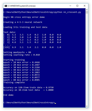
A good way to see where this article is headed is to examine the screenshot of a demo program, shown in Figure 1. The demo Python program uses CE error to train a simple neural network model that can predict the species of an iris flower using the famous Iris Dataset.
 [Click on image for larger view.]
Figure 1. Python Neural Network Cross Entropy Error Demo
[Click on image for larger view.]
Figure 1. Python Neural Network Cross Entropy Error Demo
Behind the scenes I’m using the Anaconda (version 4.1.1) distribution that contains Python 3.5.2 and NumPy 1.11.1, which are also used by Cognitive Toolkit and TensorFlow at the time I'm writing this article. The Iris Dataset has 150 items. Each item has four numeric predictor variables (often called features): sepal (a leaf-like structure) length and width, and petal length and width, followed by the species ("setosa," "versicolor" or "virginica"). The demo program uses 1-of-N label encoding so setosa = (1,0,0), versicolor = (0,1,0) and virginica = (0,0,1). The goal is to predict species from sepal and petal length and width.
The full 150-item dataset has 50 setosa items, followed by 50 versicolor, followed by 50 virginica. Before writing the demo program, I created a 120-item file of training data (using the first 30 of each species) and a 30-item file of test data (the leftover 10 of each species).
The demo program creates a simple neural network with four input nodes (one for each feature), five hidden processing nodes (the number of hidden nodes is a free parameter and must be determined by trial and error) and three output nodes (corresponding to encoded species). Although it can't be seen in the demo run screenshot, the demo neural network uses the hyperbolic tangent function for hidden node activation, and the softmax function to coerce the output nodes to sum to 1.0 so they can be interpreted as probabilities. The demo loaded the training and test data into two matrices, and then displayed the first few training items.
The demo uses the back-propagation training algorithm with CE error. The back-propagation algorithm is iterative and you must supply a maximum number of iterations (80 in the demo) and a learning rate (0.010) that controls how much each weight and bias value changes in each iteration. The max-iteration and learning rate are free parameters.
The demo displays the value of the CE error, every 10 iterations during training. Understanding the relationship between back-propagation and cross entropy is the main goal of this article. After training completed, the demo computed the classification accuracy of the resulting model on the training data (0.9750 = 117 out of 120 correct) and on the test data (1.0000 = 30 out of 30 correct). In non-demo scenarios, the classification accuracy on your test data is a very rough approximation of the accuracy you'd expect to see on new, previously unseen data.
This article assumes you understand the neural network input-output mechanism, and have at least a rough idea of how back-propagation works, but does not assume you know anything about CE error. The demo program is too long to present in its entirety in this article, but the complete source code is available in the accompanying file download.
Understanding CE Error
If you look up "cross entropy" on the Internet, one of the difficulties in understanding CE is that you'll find several different kinds of explanations. Additionally, CE error is also called "log loss" (the two terms are ever so slightly different but from an engineering point of view, the difference isn’t important). From a purely mathematical perspective, CE is an error metric that compares a set of predicted probabilities with a set of predicted probabilities. From a neural network perspective, CE is an error metric that compares a set of computed NN output nodes with values from training data. Both forms of CE are really the same, but the two different contexts can make the forms look different.
A concrete example is the best way to explain the purely mathematical form of CE. Suppose you have a weirdly shaped four-sided dice (yes, I know the singular is really "die"). Using some sort of intuition or physics, you predict that the probabilities of the four sides are (0.20, 0.40, 0.30, 0.10). Then you roll the dice many thousands of times and determine that the true probabilities are (0.15, 0.35, 0.25, 0.25). The CE error for your prediction is:
-1.0 * [ ln(0.20) * 0.15 + ln(0.40) * 0.35 + ln(0.30) * 0.25 + ln(0.10) * 0.25 ] =
-1.0 * [ (-1.61)(0.15) + (-0.92)(0.35) + (-1.20)(0.25) + (-2.30)(0.25) ] =
1.44
In words, mathematical CE error is the negative of the sum of the product of the natural log of each predicted probability times the associated actual probability. Notice that in general a perfect set of predictions doesn't give you a CE error of 0.0 and that you have to be careful not to try and calculate the ln(0.0), which is negative infinity. (All such error checking has been removed from the demo program).
Now consider CE in the context of neural network training. Suppose, for a given set of neural network weights and biases and four input values for a versicolor iris flower, the three output node values are (0.15, 0.60, 0.25). These are predicted probabilities. Because the flower is versicolor, the actual probabilities are (0, 1, 0). Therefore, CE error for this training item is:
-1.0 * [ ln(0.15) * 0 + ln(0.60) * 1 + ln(0.25) * 0) ] =
-1.0 * [ 0.00 + (-0.51)(1) + 0.00 ] =
0.51
Notice that for neural network classification, the actual probabilities (training data encoded label) will have one 1.0 value and all the others will be 0.0 values. Therefore, when computing CE error for neural network classification, only one output node value is used. If you're new to CE this may be surprising. Also, in a neural network context, a perfect prediction does in fact give you a CE error of 0.0.
The example just described is the CE error for a single training item. When training a neural network, it's common to sum the CE errors for all training items then divide by the number of training items to give an average, or mean, cross entropy error (MCEE).
The other primary error metric used for neural network training is squared error (SE). Suppose, as previously stated, predicted probabilities (the computed output node values) are (0.15, 0.60, 0.25) and actual probabilities (the training data encoded label) are (0, 1, 0). The squared error is:
(0.15 - 0)^2 + (0.60 - 1)^2 + (0.25 - 0)^2 =
0.0225 + 0.1600 + 0.0625 =
0.2450
Notice that all neural network output node values participate in the calculation of SE, and a perfect prediction gives an SE of 0.0. Just like CE, it's usual to compute a mean squared error (MSE) across all training items. As a last note, you'll find many resources on the Internet that explain CE in the context of a binary probability problem. If y* is the predicted probability that the outcome is 1, then 1 - y* is the probability that the outcome is 0. And if y is the actual probability that the outcome is 1, then the CE equation reduces to CE = - [ ln(y*)(y) + ln(1-y*)(1-y) ], which at first glance doesn't look the same as the other forms of CE even though they’re identical mathematically.
CE, SE and Back Propagation
Now that you have a solid grasp of exactly what CE is, the next step is to understand the connection between CE error and the back-propagation training algorithm. The end result is remarkably simple even though the underlying ideas are very deep.
In extremely high-level pseudo-code (meaning tons of important details left out), the back-propagation training algorithm for a simple neural network classifier with just one hidden layer is:
loop n times
  for-each training item
    1. compute gradient of each hidden-to-output weight
    2. using above, compute gradient each input-to-hidden weight
    3. using gradients, compute weight increments
    4. using increments, update all weights
  end for-each
end loop
Step No. 1 here involves calculating the Calculus derivative of the output activation function, which is almost always softmax for a neural network classifier. For ordinary SE, Python code looks like:
# compute output node signals
for k in range(self.no):
  derivative = (1 - self.oNodes[k]) * self.oNodes[k]
  oSignals[k] = derivative * (t_values[k] - self.oNodes[k])

# hidden-to-output gradients using output signals
for j in range(self.nh):
  for k in range(self.no):
    hoGrads[j,k] = oSignals[k] * self.hNodes[j]
The output signals array, oSignals, is just an intermediate convenience. The key line of code is the derivative computation. For softmax with SE, if y is a computed output node value, then the derivative is (1 - y)(y). This isn't at all obvious. You can find many explanations on the Internet.
Calculating the gradients of the input-to-hidden weights is much trickier. But if the hidden node activation function is tanh, then the key line of code is:
derivative = (1 - self.hNodes[j]) * (1 + self.hNodes[j])
If h is a computed hidden node value using tanh, then the derivative is (1 - h)(1 + h). Important alternative hidden layer activation functions are logistic sigmoid and rectified linear units, and each has a different associated derivative term.
Now here comes the really fascinating part. If, instead of using SE, you use CE error, because of some amazing algebra coincidences (well, they're not really coincidences) when you compute the gradient of the hidden-to-output weights, several terms cancel out and the derivative becomes 1. If you examine the pervious code snippet, because you multiply by the derivative, the derivative term for hidden-to-output weights essentially just goes away!
When using CE, the derivative for the input-to-hidden weight gradients does not explicitly change. However, because the input-to-hidden weight gradients are influenced by the values of the hidden-to-output gradients, the input-to-hidden gradients are indirectly changed when using CE instead of SE.
Notice that when using back propagation, you don’t need to explicitly compute either CE or SE -- the calculations are implicit in the algorithm. However, you can write a method that does explicitly calculate CE or SE so you can display the error values during training.
Comparing CE and SE
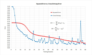
I coded up a demo program using Cognitive Toolkit with the Python and NumPy APIs. I ran the demo once using SE, and then modified the code and ran it again using CE error. The results are shown in Figure 2.
 [Click on image for larger view.]
Figure 2. Back-Propagation Update for Hidden-to-Output Weights
[Click on image for larger view.]
Figure 2. Back-Propagation Update for Hidden-to-Output Weights
The question you're probably most concerned with is, "OK, so you can use CE or SE. Which is better?" There's no clear answer -- each has pros and cons. However, the general thought among most (but definitely not all) machine learning researchers is that CE is slightly preferable to SE.
If you examine the graph in Figure 2 you can see that in this example, training with SE converges to a set of good weights and biases a bit more slowly but with less volatility than training with CE. This should make sense to you. Because SE has a derivative = (1 - y)(y) term, and y is between 0 and 1, the term will always be between 0.0 and 0.25. With CE, the derivative goes away. Very loosely, when training with SE, each weight update is about one-fourth as large as an update when training with CE.
Experimental results comparing SE and CE are inconclusive in my opinion. However, most machine learning researchers "have a love affair with CE error" as one of my research colleagues phrased it in an informal chat near our workplace coffee machine recently. There’s some rather subjective reasoning that can be used to justify a preference for using CE. You can find a handful of research papers that discuss the argument by doing an Internet search for "pairing softmax activation and cross entropy." Basically, the idea is that there’s a nice mathematical relation between CE and softmax that doesn't exist between SE and softmax.
Overall Demo Program Structure
The overall demo program structure is presented in Listing 1. To edit the demo program, I used the simple Notepad program. Yes, Notepad. I like Notepad. Most of my colleagues prefer using one of the many nice Python editors that are available.
I added three import statements to gain access to the NumPy package's array and matrix data structures, and the math and random modules. Function loadFile reads either training or test, comma-delimited data into a NumPy array-of-arrays style matrix. (Instead of using the program-defined loadFile function, you also could use the built-in NumPy loadtxt function.) The show_ functions are just helpers to display floating point data with a specified number of decimals.
Listing 1: Cross Entropy Error Demo in Python
# nn_crossent.py
# Anaconda 4.1.1
# (Python 3.5.2 and NumPy 1.11.1)

import numpy as np
import random
import math

def loadFile(df):
def showVector(v, dec):
def showMatrix(m, dec):
def showMatrixPartial(m, numRows, dec, indices):

# -----
class NeuralNetwork:
  def __init__(self, numInput, numHidden, numOutput):
  def setWeights(self, weights):
  def getWeights(self):
  def initializeWeights(self):
  def computeOutputs(self, xValues):
  def train(self, trainData, maxEpochs, learnRate):
  def accuracy(self, tdata):
  def meanCrossEntropyError(self, tdata):
  def meanSquaredError(self, tdata):

  @staticmethod
  def hypertan(x):

  @staticmethod
  def softmax(oSums):

  @staticmethod
  def totalWeights(nInput, nHidden, nOutput):
# -----

def main():
  print("\nBegin NN cross entropy error demo \n")

  numInput = 4
  numHidden = 5
  numOutput = 3
  print("Creating a %d-%d-%d neural network " % \
    (numInput, numHidden, numOutput) )
  nn = NeuralNetwork(numInput, numHidden, numOutput)

  print("\nLoading Iris training and test data ")
  trainDataPath = "irisTrainData.txt"
  trainDataMatrix = loadFile(trainDataPath)
  print("\nTest data: ")
  showMatrixPartial(trainDataMatrix, 4, 1, True)
  testDataPath = "irisTestData.txt"
  testDataMatrix = loadFile(testDataPath)

  maxEpochs = 80
  learnRate = 0.01
  print("\nSetting maxEpochs = " + str(maxEpochs))
  print("Setting learning rate = %0.3f " % learnRate)
  print("\nStarting training")
  nn.train(trainDataMatrix, maxEpochs, learnRate)
  print("Training complete")

  accTrain = nn.accuracy(trainDataMatrix)
  accTest = nn.accuracy(testDataMatrix)

  print("\nAccuracy on 120-item train data = \
    %0.4f " % accTrain)
  print("Accuracy on 30-item test data   = \
    %0.4f " % accTest)

  print("\nEnd demo \n")

if __name__ == "__main__":
  main()

# end script
The key method is NeuralNetwork.train and it implements back-propagation training with CE error. I created a main function to hold all program control logic. I started by creating a 4-5-3 neural network, like so:
def main():
  numInput = 4
  numHidden = 5
  numOutput = 3
  nn = NeuralNetwork(numInput, numHidden, numOutput)
...
The class uses a hardcoded tanh hidden layer activation and the constructor sets a class-scope random number generator seed so results will be reproducible. All weights and biases are initialized to small random values between -0.01 and +0.01. Next, I loaded training and test data into memory with these statements:
trainDataPath = "irisTrainData.txt"
trainDataMatrix = loadFile(trainDataPath)
testDataPath = "irisTestData.txt"
testDataMatrix = loadFile(testDataPath)
The back-propagation training is prepared and invoked:
maxEpochs = 80
learnRate = 0.01
nn.train(trainDataMatrix, maxEpochs, learnRate)
Method train uses the back-propagation algorithm and displays a progress message with the current CE error, every 10 iterations. It's usually important to monitor progress during neural network training because it's not uncommon for training to stall out completely, and if that happens you don't want to wait for an entire training run to complete. The demo program concludes with these statements:
...
  accTrain = nn.accuracy(trainDataMatrix)
  accTest = nn.accuracy(testDataMatrix)

  print("\nAccuracy on 120-item train data = \
    %0.4f " % accTrain)
  print("Accuracy on 30-item test data   = \
    %0.4f " % accTest)

  print("\nEnd demo \n")

if __name__ == "__main__":
  main()

# end script
Notice that during training you’re primarily interested in error, but after training you’re primarily interested in classification accuracy.
Wrapping Up
To recap, when performing neural network classifier training, you can use squared error or cross entropy error. Cross entropy is a measure of error between a set of predicted probabilities (or computed neural network output nodes) and a set of actual probabilities (or a 1-of-N encoded training label). Cross entropy error is also known as log loss. Squared error is a more general form of error and is just the sum of the squared differences between a predicted set of values and an actual set of values. Often, when using back-propagation training, cross entropy tends to give better training results more quickly than squared error, but squared error is less volatile than cross entropy.
In my opinion, research results about which error metric gives better results are inconclusive. In the early days of neural networks, squared error was the most common error metric, but currently cross entropy is used more often. There are other error metrics that can be used for neural network training, but there’s no solid research on this topic of which I'm aware.