The Data Science Lab
Neural Network Momentum Using Python
With the help of Python and the NumPy add-on package, I'll explain how to implement back-propagation training using momentum.
Neural network momentum is a simple technique that often improves both training speed and accuracy. Training a neural network is the process of finding values for the weights and biases so that for a given set of input values, the computed output values closely match the known, correct, target values. For example, suppose you’re trying to predict the species of an iris flower (setosa, versicolor or viriginica) based on the flower's sepal length, sepal width, petal length and petal width.
If you encode setosa as (1, 0, 0) and versicolor as (0, 1, 0) and virginica as (0, 0, 1), then a neural network classifier would have four input nodes and three output nodes. If your network has five hidden processing nodes, then the network has (4 * 5) + (5 * 3) = 35 weights and (5 + 3) = 8 biases that must be determined.
Suppose a set of input values for one training item is (5.1, 3.5, 1.4, 0.2) and the correct species is (1, 0, 0). If the computed output node values are (0.65, 0.20, 0.15), then a training algorithm needs to adjust the 43 weights and biases values so the value of the first output node increases and the values of the other two output nodes decrease.
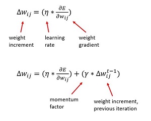
The most common training technique is to use the back-propagation algorithm. If you update all the weights and biases after processing a single training item ("stochastic" or "online" training), the basic update rule, without using momentum, for a single weight is shown as the top formula in Figure 1. In words, "the delta increment for the weight connecting node i to node j equals a learning rate constant times the gradient associated with the weight."
 [Click on image for larger view.]
Figure 1. Back-Propagation Update Without and with Momentum
[Click on image for larger view.]
Figure 1. Back-Propagation Update Without and with Momentum
During training, suppose a weight currently has a value of 3.85 and the learning rate is set to 0.10. If, for a set of input and computed output values, the gradient associated with the weight is computed to be 7.60, then the weight delta is 0.10 * 7.60 = 0.76 and so the new value of the weight is 3.85 + 0.76 = 4.61.
Using momentum, the modified update rule is shown as the bottom formula in Figure 1. In words, "the weight delta equals the learning rate times the gradient, plus a momentum factor times the weight delta from the previous iteration." For example, if during training a weight has a value of 3.56, the learning rate is set to 0.10, the computed gradient is 4.70, the momentum factor is set to 0.50, and the value of the weight delta from the previous training iteration was 0.62, then the weight delta is (0.10 * 4.70) + (0.50 * 0.62) = 0.47 + 0.31 = 0.78, and so the new value of the weight is 3.56 + 0.78 = 4.34.
In this article I'll explain how to implement back-propagation training using momentum. I use Python with the NumPy add-on package. After reading this article you should have a solid grasp of back-propagation using momentum, as well as knowledge of Python and NumPy techniques that can be useful when working with libraries such as CNTK and TensorFlow.
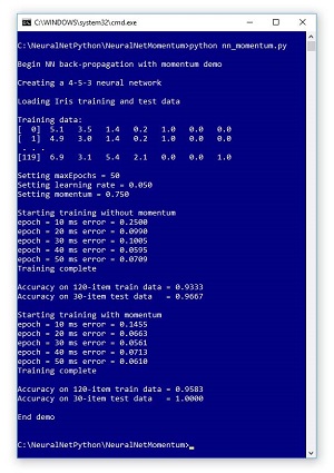
A good way to see where this article is headed is to take a look at the screenshot of a demo program in Figure 2. The demo Python program uses back-propagation both with and without momentum. The famous Fisher's Iris Dataset has 150 items. Each item has four numeric predictor variables (sometimes called features): sepal length and width, and petal length and width, followed by the species where setosa = (1,0,0) and versicolor = (0,1,0) and virginica = (0,0,1). The goal is to predict species from sepal and petal length and width.
 [Click on image for larger view.]
Figure 2. Python Neural Network Momentum Demo
[Click on image for larger view.]
Figure 2. Python Neural Network Momentum Demo
The complete 150-item dataset has 50 setosa items, followed by 50 versicolor, followed by 50 virginica. Before writing the demo program, I created a 120-item file of training data (using the first 30 of each species) and a 30-item file of test data (the remaining 10 of each species).
The demo program creates a simple neural network with four input nodes, five hidden processing nodes (the number of hidden nodes is a free parameter and must be determined by trial and error) and three output nodes. The demo loaded the training and test data into two matrices.
The back-propagation algorithm is iterative, and you must supply a maximum number of iterations (50 in the demo). The learning rate was set to 0.050, and the momentum factor was set to 0.750. These are free parameters, and the values were determined by trial and error.
In the first run, no momentum was used. In the second demo run, momentum was used. If you examine the outputs, you'll see that the demo run using momentum converged toward small error more quickly (0.0610 vs 0.0707), and resulted in better prediction accuracy (95.83 percent vs. 93.33 percent) than the demo run without using momentum.
This article assumes you have a solid knowledge of the neural network input-output mechanism and intermediate or better programming skills with a C-family language (C#, Python, Java), but doesn’t assume you know anything about momentum with the back-propagation algorithm. The demo program is too long to present in its entirety in this article, but the complete source code is available in the accompanying file download.
Overall Demo Program Structure
The overall demo program structure is presented in Listing 1. To edit the demo program, I used Notepad. You might prefer to use one of the many nice Python editors available. I indented the demo using two spaces rather than the more-common four spaces to save space.
I commented the name of the program and indicated that I'm using Python 3. I added three import statements to gain access to the NumPy package's array and matrix data structures, and the math and random modules.
Listing 1: Overall Program Structure
# nn_momentum.py
# Python 3.x

import numpy as np
import random
import math

# ------------------------------------

def showVector(v, dec): ...
def showMatrixPartial(m, numRows, dec, indices): ...

# ------------------------------------

class NeuralNetwork: ...

# ------------------------------------

def main():
  print("\nBegin NN back-propagation with momentum demo \n")

  numInput = 4
  numHidden = 5
  numOutput = 3
  seed = 3
  print("Creating a %d-%d-%d neural network " %
   (numInput, numHidden, numOutput) )
  nn = NeuralNetwork(numInput, numHidden, numOutput, seed)

  print("\nLoading Iris training and test data ")
  trainDataPath = "irisTrainData.txt"
  trainDataMatrix = np.loadtxt(trainDataPath,
    dtype=np.float32, delimiter=",")
  print("\nTrain data: ")
  showMatrixPartial(trainDataMatrix, 2, 1, True)
  testDataPath = "irisTestData.txt"
  testDataMatrix = np.loadtxt(testDataPath,
    dtype=np.float32, delimiter=",")

  maxEpochs = 50
  learnRate = 0.05
  momentum = 0.75
  print("\nSetting maxEpochs = " + str(maxEpochs))
  print("Setting learning rate = %0.3f " % learnRate)
  print("Setting momentum = %0.3f " % momentum)

  print("\nStarting training without momentum")
  nn.train(trainDataMatrix, maxEpochs, learnRate, 0.0)
  print("Training complete")

  accTrain = nn.accuracy(trainDataMatrix)
  accTest = nn.accuracy(testDataMatrix)

  print("\nAccuracy on 120-item train data = %0.4f "
    % accTrain)
  print("Accuracy on 30-item test data   = %0.4f "
    % accTest)

  nn = NeuralNetwork(numInput, numHidden, numOutput, seed)
  print("\nStarting training with momentum")
  nn.train(trainDataMatrix, maxEpochs, learnRate, momentum)
  print("Training complete")

  accTrain = nn.accuracy(trainDataMatrix)
  accTest = nn.accuracy(testDataMatrix)

  print("\nAccuracy on 120-item train data = %0.4f "
    % accTrain)
  print("Accuracy on 30-item test data   = %0.4f "
    % accTest)

  print("\nEnd demo \n")

if __name__ == "__main__":
  main()

# end script
The demo program consists mostly of a program-defined NeuralNetwork class. I used a main function to hold all program control logic. I started by creating the neural network like so:
def main():
  print("Begin NN momentum demo ")
  numInput = 4
  numHidden = 5
  numOutput = 3
  seed = 3
  print("Creating a %d-%d-%d neural network " %
   (numInput, numHidden, numOutput) )
  nn = NeuralNetwork(numInput, numHidden,
    numOutput, seed)
...
The seed value passed to the neural network constructor controls weight and bias initial values and the random ordering in which training items are processed. The value I used, 3, was selected only because it gave representative demo results. Next, I loaded the training and test data:
print("Loading Iris training and test data ")
trainDataPath = "irisTrainData.txt"
trainDataMatrix = np.loadtxt(trainDataPath,
  dtype=np.float32, delimiter=",")
print("Training data: ")
showMatrixPartial(trainDataMatrix, 2, 1, True)
testDataPath = "irisTestData.txt"
testDataMatrix = np.loadtxt(testDataPath,
  dtype=np.float32, delimiter=",")
The NumPy loadtxt function is very convenient and returns an array of arrays style matrix. I used float32 data because, in general, neural networks don't need 64-bit floating-point precision. Next, I prepared training:
maxEpochs = 50
learnRate = 0.05
momentum = 0.75
print("Setting maxEpochs = " + str(maxEpochs))
print("Setting learning rate = %0.3f "
  % learnRate)
print("Setting momentum = %0.3f " % momentum)
The demo performs training without momentum using these statements:
print("Starting training without momentum")
nn.train(trainDataMatrix, maxEpochs,
  learnRate, 0.0)
print("Training complete")
accTrain = nn.accuracy(trainDataMatrix)
accTest = nn.accuracy(testDataMatrix)
print("Accuracy on 120-item train data = %0.4f "
  % accTrain)
print("Accuracy on 30-item test data = %0.4f "
  % accTest)
The train method has four parameters. The fourth is the momentum factor. If you refer to the second formula in Figure 1, you'll see that by setting the momentum factor to 0.0, the part of the weight delta due to momentum drops out. Easy! The demo performs training with momentum like this:
nn = NeuralNetwork(numInput, numHidden,
  numOutput, seed)
print("Starting training with momentum")
nn.train(trainDataMatrix, maxEpochs,
  learnRate, momentum)
print("Training complete")
accTrain = nn.accuracy(trainDataMatrix)
accTest = nn.accuracy(testDataMatrix)
print("Accuracy on 120-item train data = %0.4f "
  % accTrain)
print("Accuracy on 30-item test data = %0.4f "
  % accTest)
print("End demo ")
It's important to reset the neural network by calling the constructor, otherwise you'd start training with the good weights and bias values found from the previous training.
The Training Method
The NeuralNetwork.train method implements online/stochastic back-propagation using momentum. In very high-level pseudo-code, the training algorithm is:
loop maxEpochs times
  for-each training item
    compute output, hidden node signals
    compute weight gradients
    compute weight deltas and save
    update weights using gradients
    update weights using momentum
  end-for
end-loop
The method implementation begins:
def train(self, trainData, maxEpochs, learnRate):
  hoGrads = np.zeros(shape=[self.nh, self.no],
    dtype=np.float32)
  obGrads = np.zeros(shape=[self.no],
    dtype=np.float32)
  ihGrads = np.zeros(shape=[self.ni, self.nh],
    dtype=np.float32)
  hbGrads = np.zeros(shape=[self.nh],
    dtype=np.float32)
...
Each weight and bias has an associated gradient. The prefix "ho" stands for "hidden-to-output". Similarly, "ob" means "output bias," "ih" means "input-to-hidden" and "hb" means "hidden bias." Class members ni, nh, and no are the number of input, hidden, and output nodes, respectively. When working with neural networks, it's common, but not required, to work with float32 data.
Next, two scratch arrays are instantiated:
oSignals = np.zeros(shape=[self.no], dtype=np.float32)
hSignals = np.zeros(shape=[self.nh], dtype=np.float32)
Each hidden and output node has an associated signal that is the gradient without its input term. These arrays are mostly for coding convenience because they're used twice. Next, storage for each weight and bias delta from the previous iteration are set up:
ih_prev_weights_delta = np.zeros(shape=[self.ni,
  self.nh], dtype=np.float32)
h_prev_biases_delta = np.zeros(shape=[self.nh],
  dtype=np.float32)
ho_prev_weights_delta = np.zeros(shape=[self.nh,
  self.no], dtype=np.float32)
o_prev_biases_delta = np.zeros(shape=[self.no],
  dtype=np.float32)
The main training loop is prepared like so:
epoch = 0
x_values = np.zeros(shape=[self.ni], dtype=np.float32)
t_values = np.zeros(shape=[self.no], dtype=np.float32)
numTrainItems = len(trainData)
indices = np.arange(numTrainItems)
The x_values and t_values arrays hold a set of feature values (sepal length and width, and petal length and width) and target values (such as 1, 0, 0), respectively. The indices array hold integers 0 through 119 and is used to shuffle the order in which training items are processed -- very important when using the online/stochastic approach. The training loop begins with:
while epoch < maxEpochs:
  self.rnd.shuffle(indices)
  for ii in range(numTrainItems):
    idx = indices[ii]
...
The built-in Python shuffle function scrambles the order of the training indices. Therefore, variable idx points to the current training item being processed. Inside the main loop, the input and target values are peeled off the current training item, and then the output node values are computed using the input values and the current weights and bias values:
for j in range(self.ni):
  x_values[j] = trainData[idx, j]
for j in range(self.no):
  t_values[j] = trainData[idx, j+self.ni]
self.computeOutputs(x_values)
Note that there is an array-slicing shortcut idiom specific to Python you could use here. I avoided it in case you want to refactor the demo code to a language that doesn't support slicing. The first step in back-propagation is to compute the output node signals:
# 1. compute output node signals
for k in range(self.no):
  derivative = (1 - self.oNodes[k]) * self.oNodes[k]
  oSignals[k] = derivative * (self.oNodes[k] - t_values[k])
The value for the variable named derivative assumes you have a neural network classifier that uses softmax activation. To compute the signal, the demo assumes the goal is to minimize mean squared error and uses "output minus target" rather than "target minus output," which would change the sign of the weight delta. Next, the hidden-to-output weight gradients are computed:
# 2. compute hidden-to-output weight gradients
for j in range(self.nh):
  for k in range(self.no):
    hoGrads[j, k] = oSignals[k] * self.hNodes[j]
The output node signal is combined with the associated input from the associated hidden node to give the gradient. Next, the gradients for the output node biases are computed:
# 3. compute output node bias gradients
for k in range(self.no):
  obGrads[k] = oSignals[k] * 1.0
You can think of a bias as a special kind of weight that has a constant, dummy 1.0 associated input. Here I use an explicit 1.0 value only to emphasize that idea, so you can omit it if you wish. Next, the hidden node signals are computed:
# 4. compute hidden node signals
for j in range(self.nh):
  sum = 0.0
  for k in range(self.no):
    sum += oSignals[k] * self.hoWeights[j,k]
  derivative = (1 - self.hNodes[j]) * (1 + self.hNodes[j])
  hSignals[j] = derivative * sum
The demo neural network uses the tanh activation function for hidden nodes. The local variable named derivative holds the calculus derivative of the tanh function. So, if you change the hidden node activation function, you'd have to change the calculation of this derivative variable. Next, the input-to-hidden weight gradients and the hidden node bias gradients are calculated:
# 5. compute input-to-hidden weight gradients
for i in range(self.ni):
  for j in range(self.nh):
    ihGrads[i, j] = hSignals[j] * self.iNodes[i]

# 6. compute hidden node bias gradients
for j in range(self.nh):
  hbGrads[j] = hSignals[j] * 1.0
As before, a gradient is composed of a signal and an associated input term, and the dummy 1.0 input value for the hidden biases can be dropped. Notice that the code hasn't used momentum yet. After the gradients have been calculated, the weight and bias values can be updated in any order. First, the demo updates the input-to-hidden node weights:
# 1. update input-to-hidden weights
for i in range(self.ni):
  for j in range(self.nh):
    delta = -1.0 * learnRate * ihGrads[i,j]
    self.ihWeights[i,j] += delta
    self.ihWeights[i,j] += momentum * ih_prev_weights_delta[i,j]
    ih_prev_weights_delta[i,j] = delta
After the weight delta is calculated, the weight is updated. Then a second update is performed using the value of the previous delta. In the very first training iteration, the initial value of the weight delta will be 0.0, but that's fine. Before exiting the loop, the previous delta is replaced by the current delta value.
Next, the hidden node biases are updated in the same way:
# 2. update hidden node biases
for j in range(self.nh):
  delta = -1.0 * learnRate * hbGrads[j]
  self.hBiases[j] += delta
  self.hBiases[j] += momentum * h_prev_biases_delta[j]
  h_prev_biases_delta[j] = delta
Next, the hidden-to-output weights and the output node biases are updated using the same pattern:
# 3. update hidden-to-output weights
for j in range(self.nh):
  for k in range(self.no):
    delta = learnRate * hoGrads[j,k]
    self.hoWeights[j,k] += delta
    self.hoWeights[j,k] += momentum * ho_prev_weights_delta[j,k]
    ho_prev_weights_delta[j,k] = delta

# 4. update output node biases
for k in range(self.no):
  delta = learnRate * obGrads[k]
  self.oBiases[k] += delta
  self.oBiases[k] += momentum * o_prev_biases_delta[k]
  o_prev_biases_delta[k] = delta
Notice that all updates use the same fixed learning rate. Advanced versions of back-propagation use adaptive learning rates that change. The main training loop finishes by updating the iteration counter and printing a progress message, and then method NeuralNetwork.train wraps up like so:
...
    epoch += 1
    if epoch % 10 == 0:
      mse = self.meanSquaredError(trainData)
      print("epoch = " + str(epoch) + " ms error = %0.4f " % mse)
  # end while

  result = self.getWeights()
  return result
# end train
Here, a progress message with the current mean squared error is displayed every 10 iterations. You might want to parameterize the interval. You can also print additional diagnostic information here. The final values of the weights and biases are fetched by class method getWeights and returned by method train as a convenience.
Wrapping Up
Momentum is almost always used when training a neural network with back-propagation. Exactly why momentum is so effective is a bit subtle. Suppose in the early stages of training a weight delta is calculated to be +4.32, and then on the next iteration the delta for the same weight is calculated to be +3.95. Training is "headed in the right direction" so to speak, and momentum adds a boost to the weight change, which makes training faster. Suppose in the middle stages of training the weight deltas start oscillating between positive and negative values. Using momentum will dampen the oscillation, making the resulting model more accurate.
Momentum isn’t a cure-all. When training a neural network, you must experiment with different momentum factor values. In some situations, using no momentum (or equivalently, a momentum factor of 0.0) leads to better results than using momentum. However, in most scenarios, using momentum gives you faster training and better predictive accuracy.
About the Author
Dr. James McCaffrey directs the data science and research efforts at Quaetrix, a data analytics company located near Redmond, Washington. Before joining Quaetrix, James was a senior research engineer at Microsoft. James can be reached at [email protected].