The Data Science Lab
Data Clustering with K-Means Using Python
Data clustering, or cluster analysis, is the process of grouping data items so that similar items belong to the same group/cluster. There are many clustering techniques. In this article I'll explain how to implement the k-means technique.
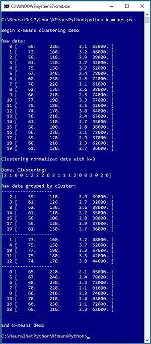
Take a look at the screenshot in Figure 1. The demo program reads 20 data items into memory. Each item represents a person's height in inches, weight in pounds, high school GPA and annual income. Even with only 20 items, it's difficult to see any pattern.
 [Click on image for larger view.]
Figure 1. Clustering Using the K-Means Technique
[Click on image for larger view.]
Figure 1. Clustering Using the K-Means Technique
The demo program sets the number of clusters, k, to 3. When performing cluster analysis, you must manually specify the number of clusters to use. After clustering, the results are displayed as an array: (2 1 0 0 1 2 . . . 0). A cluster ID is just an integer: 0, 1 or 2. The results mean data item [0] belongs to cluster 2, item [1] belongs to cluster 1, item [2] belongs to cluster 0 and so on, to item [19] which belongs to cluster 0. The demo displays the raw data, grouped by cluster ID, and you can see a clear pattern.
Although many machine learning code libraries have a clustering function, implementing a custom clustering function is relatively easy and gives you complete control over the many options that are possible.
This article assumes you have intermediate or better programming skill with a C-family language but doesn't assume you know anything about the k-means technique. The complete demo code is presented in this article. All normal error-checking has been removed to keep the main ideas as clear as possible.
The Demo Program Structure
The structure of the demo program, with a few minor edits to save space, is presented in Listing 1. I indent two spaces rather than the usual four spaces as a matter of personal preference and to save space. The contents of the raw data file are presented in Listing 2.
Listing 1: Clustering with K-Means Program Structure
# k_means.py
# Anaconda 4.1.1
import numpy as np

def mm_normalize(data): . . .
def distance(item, mean): . . .
def update_clustering(norm_data, clustering, means): . . .
def update_means(norm_data, clustering, means): . . .
def initialize(norm_data, k): . . .
def cluster(norm_data, k): . . .
def display(raw_data, clustering, k): . . .

def main():
  print("\nBegin k-means clustering demo \n")
  np.set_printoptions(precision=4, suppress=True)
  np.random.seed(2)

  raw_data = np.loadtxt(".\\ht_wt_gpa_inc.txt", dtype=np.float32,
    delimiter=",", skiprows=0, usecols=[0,1,2,3])
  (n, dim) = raw_data.shape

  print("Raw data:")
  for i in range(n):
    print("%4d " % i, end=""); print(raw_data[i])

  (norm_data, mins, maxs) = mm_normalize(raw_data)

  k = 3
  print("\nClustering normalized data with k=" + str(k))
  clustering = cluster(norm_data, k)

  print("\nDone. Clustering:")
  print(clustering)

  print("\nRaw data grouped by cluster: ")
  display(raw_data, clustering, k)

  print("\nEnd k-means demo ")

if __name__ == "__main__":
  main()
The demo uses Python 3.5 in the Anaconda 4.1.1 distribution. The program imports the NumPy package to gain access to array functionality. The demo defines seven helper methods, which will be explained shortly.
The main() function begins by loading the raw data from a text file into memory:
  np.random.seed(2)
  raw_data = np.loadtxt(".\\ht_wt_gpa_inc.txt", dtype=np.float32,
    delimiter=",", skiprows=0, usecols=[0,1,2,3])
  (n, dim) = raw_data.shape
  print("Raw data:")
  for i in range(n):
    print("%4d " % i, end=""); print(raw_data[i])
The k-means technique has an element of randomness, so the random seed is set so that results are reproducible. The loadtxt() function is a very convenient way to load numeric data into a NumPy array-of-arrays style matrix. For many machine learning problems, using 32-bit floating point values is preferred to using 64-bit values because the extra precision isn't needed. The shape property gives the number of rows (20) and columns (4) of the result matrix, as a Python tuple.
Next, the demo normalizes the raw data:
(norm_data, mins, maxs) = mm_normalize(raw_data)
The program-defined mm_normalize() function returns a matrix where the values have been normalized using the min-max technique. An array holding the minimum raw value in each column, and an array holding the maximum raw value in each column, are also returned. It is almost always essential to normalize data before clustering. Without normalization, large values, such as annual incomes in the demo, would overwhelm small values, such as GPA.
Listing 2: Contents of ht_wt_gpa_inc.txt
65.0, 220.0, 2.1, 65000.00
73.0, 160.0, 3.2, 48000.00
59.0, 110.0, 2.9, 39000.00
61.0, 120.0, 2.7, 32000.00
75.0, 150.0, 3.7, 52000.00
67.0, 240.0, 2.4, 78000.00
68.0, 230.0, 2.3, 72000.00
70.0, 220.0, 2.1, 61000.00
62.0, 130.0, 2.6, 38000.00
66.0, 210.0, 2.3, 74000.00
77.0, 190.0, 3.3, 57000.00
75.0, 180.0, 3.5, 42000.00
74.0, 170.0, 3.8, 44000.00
70.0, 210.0, 2.4, 63000.00
61.0, 110.0, 2.7, 35000.00
58.0, 100.0, 2.8, 38000.00
66.0, 230.0, 2.1, 72000.00
59.0, 120.0, 2.9, 37000.00
68.0, 210.0, 2.3, 62000.00
61.0, 130.0, 2.7, 36000.00
The demo performs clustering like so:
  k = 3
  print("\nClustering normalized data with k=" + str(k))
  clustering = cluster(norm_data, k)
  print("\nDone. Clustering:")
  print(clustering)
The cluster() function calls helpers initialize(), update_clustering() and update_means(). Function update_clustering() calls function distance().
Distances and Means
To understand the k-mean clustering technique, you must have a solid grasp of the meaning of the distance between two vectors, and the mean of a set of vectors. Both ideas are best explained by example. Suppose you have a vector v1 = (65.0, 220.0, 2.1, 65000.00) and a vector v2 = (73.0, 160.0, 3.2, 48000.00). The Euclidean distance between v1 and v1 is:
dist = sqrt( (65 - 73)^2 + (220 - 160)^2 + (2.1 - 3.2)^2 + (65000 - 48000)^2 )
       = sqrt( 64 + 3600 + 1.21 + 2.89e+8 )
       = sqrt(289003665.2)
       = 17000.11
Notice that in this example the annual income values completely dominate the calculation, which is why normalization is essential before clustering.
The demo implements the distance function as:
def distance(item, mean):
  sum = 0.0
  dim = len(item)
  for j in range(dim):
    sum += (item[j] - mean[j]) ** 2
  return np.sqrt(sum)
The mean of a set of vectors is a composite of the averages of each component. For example, if
v1 = (3.0, 6.0, 2.0, 4.0)
v2 = (1.0, 0.0, 1.0, 2.0)
v3 = (2.0, 3.0, 0.0, 6.0)
then the mean of the three vectors is:
mean = (2.0, 3.0, 1.0, 4.0)
The demo program does not define an explicit function to compute means. Function update_means() computes the means of data items assigned to each cluster on the fly.
Min-Max Normalization
To perform min-max normalization on a set of values in a column of data, you first determine the largest and smallest values in the column. Then each value v in the column is replaced by (v - min) / (max - min). For example, if a column of data had four values: (5, 8, 2, 3), then min = 2 and max = 8. The first raw value, 5, is replaced by (5 - 2) / (8 - 2) = 3 / 6 = 0.50. The normalized column values would be (0.50, 1.00, 0.00, 0.17). After min-max normalization, all normalized values will be between 0.0 and 1.0.
The demo implements a function that normalizes a NumPy matrix with:
def mm_normalize(data):
  (rows, cols) = data.shape  # (20,4)
  mins = np.zeros(shape=(cols), dtype=np.float32)
  maxs = np.zeros(shape=(cols), dtype=np.float32)
  for j in range(cols):
    mins[j] = np.min(data[:,j])
    maxs[j] = np.max(data[:,j])

  result = np.copy(data)
  for i in range(rows):
    for j in range(cols):
      result[i,j] = (data[i,j] - mins[j]) / (maxs[j] - mins[j])
  return (result, mins, maxs)
The function returns a new matrix with normalized values, an array of column min values and an array of column max values. The min and max arrays are returned in case you want to normalize a new data item so that it can be clustered with the original dataset.
The K-Means Technique
There are many variations of the k-means technique. The basic version is sometimes called Lloyd's heuristic. The demo program version in pseudo-code is:
initialize clustering assignments and means

loop until no change in clustering
  update the clustering assignments (using new means)
  update the means (using new clustering assignments)
end-loop

return clustering assignments
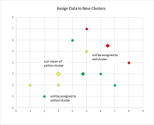
The k-means method is illustrated in Figure 2. Suppose there are just nine data items (as small circles), and each has two dimensions (for example, height and weight). And suppose at some point in the clustering iterations, the three means are indicated by the large diamonds. As each data item is processed, it will be assigned to the cluster with the closest mean. So, the item at (2, 1), currently clustered as "green," will be assigned to "yellow." And the data item at (5, 5), currently "yellow," will be assigned to cluster "red." After only a few iterations, all nine data items will be clustered nicely.
The demo program implements function cluster() as:
def cluster(norm_data, k):
  (clustering, means) = initialize(norm_data, k)
  ok = True  # if a change was made and no bad clustering
  max_iter = 100
  sanity_ct = 1
  while sanity_ct <= max_iter:
    ok = update_clustering(norm_data, clustering, means)
    if ok == False:
      break  # done
    update_means(norm_data, clustering, means)
    sanity_ct += 1
  return clustering
The update_clustering() function modifies its clustering array parameter by reference and returns True if things work, or returns False if there is no change to clustering assignments (which means the clustering has completed), or if the proposed clustering would have resulted in a set of clustering assignments where one or more clusters has no data items assigned to it.
The k-means technique typically stabilizes very quickly, often within 10 iterations. But it's good practice to put some sort of sanity-count check in place to prevent an infinite loop.
 [Click on image for larger view.]
Figure 2. The K-Means Method
[Click on image for larger view.]
Figure 2. The K-Means Method
To reiterate, to assign an item to a cluster, the item is compared against the means of each cluster and is assigned to the cluster whose mean is closest to the item. For example, suppose at some point in a clustering problem, the vector v = (2, 5, 7) must be assigned. And suppose k = 3, and the current means of the three clusters are m[0] = (9.5, 0.5, 1.5), m[1] = (2.5, 4.5, 7.0), m[2] = (8.5, 1.5, 1.5). The vector v is clearly closest to mean m[1], and so v is assigned to cluster 1.
Initializing Means and Clustering Assignments
Most of the variations of the k-means technique deal with different ways to initialize the clustering assignments and means. The demo program initially assigns each data item to a random cluster, making sure that each cluster has at least one data item in it. After each data item is assigned to a cluster, the means of the items belonging to each cluster are computed.
The demo implements function initialize() as:
def initialize(norm_data, k):
  (n, dim) = norm_data.shape
  clustering = np.zeros(shape=(n), dtype=np.int)
  for i in range(k):
    clustering[i] = i
  for i in range(k, n):
    clustering[i] = np.random.randint(0, k)

  means = np.zeros(shape=(k,dim), dtype=np.float32)
  update_means(norm_data, clustering, means)
  return(clustering, means)
An alternative initialization scheme is to randomly select k data items to act as initial means, and then assign each remaining data item to a cluster. This approach is more likely to lead to a bad clustering result than the approach used by the demo. At the other extreme, a variation called k-means++ uses a moderately complex probabilistic algorithm to initialize clustering assignments.
Updating Clustering Assignments
The update_clustering() function is presented in Listing 2. The function checks for situation where a proposed new clustering assignment would result in no change. In that case the algorithm has completed. The np.array_equal() function is handy for this purpose.
Listing 2: The update_clustering() Function
def update_clustering(norm_data, clustering, means):
  # given a (new) set of means, assign new clustering
  # return False if no change or bad clustering
  n = len(norm_data)
  k = len(means)

  new_clustering = np.copy(clustering)  # proposed clustering
  distances = np.zeros(shape=(k), dtype=np.float32)

  for i in range(n):  # walk thru each data item
    for kk in range(k):
      distances[kk] = distance(norm_data[i], means[kk])
    new_id = np.argmin(distances)
    new_clustering[i] = new_id

  if np.array_equal(clustering, new_clustering):  # no change
    return False

  # make sure that no cluster counts have gone to zero
  counts = np.zeros(shape=(k), dtype=np.int)
  for i in range(n):
    c_id = clustering[i]
    counts[c_id] += 1

  for kk in range(k):  # could use np.count_nonzero
    if counts[kk] == 0:  # bad clustering
      return False

  # there was a change, and no counts have gone 0
  for i in range(n):
   clustering[i] = new_clustering[i]  # update by ref
  return True
It is unlikely, but possible, for the k-means technique to assign data items to clusters so that a cluster has no associated data items -- an empty cluster. In most situations this is not desired behavior. So, for a proposed clustering, the demo code computes the number of data items assigned and exits if the proposed clustering would result in an empty cluster.
Updating Means
The demo implements function update_means() as shown in Listing 3. Conceptually, calculating the mean of a set of vectors is simple, but the code is a bit trickier than you might expect. It's easy to make a mistake because there is a lot of array indexing going on across several data structures.
Listing 3: The update_means() Function
def update_means(norm_data, clustering, means):
  # given a (new) clustering, compute new means
  # assumes update_clustering has just been called
  # to guarantee no 0-count clusters
  (n, dim) = norm_data.shape
  k = len(means)
  counts = np.zeros(shape=(k), dtype=np.int)
  new_means = np.zeros(shape=means.shape, dtype=np.float32)  # k x dim
  for i in range(n):  # walk thru each data item
    c_id = clustering[i]
    counts[c_id] += 1
    for j in range(dim):
      new_means[c_id,j] += norm_data[i,j]  # accumulate sum

  for kk in range(k):  # each mean
    for j in range(dim):
      new_means[kk,j] /= counts[kk]  # assumes not zero

  for kk in range(k):  # each mean
    for j in range(dim):
      means[kk,j] = new_means[kk,j]  # update by ref
Functions update_means() and update_clustering() both modify their array parameters by reference (clustering and means, respectively). An alternative is to return the new arrays and then assign. For example, means = update_means(norm_data, clustering, means) rather than just update_means(norm_data, clustering, means).
Wrapping Up
The demo program represents a set of clustering assignments as an array of integers. This array can be used to display the raw data, grouped by cluster:
def display(raw_data, clustering, k):
  (n, dim) = raw_data.shape
  print("-------------------")
  for kk in range(k):  # group by cluster ID
    for i in range(n):  # scan the raw data
      c_id = clustering[i]  # cluster ID of curr item
      if c_id == kk:
        print("%4d " % i, end=""); print(raw_data[i])
    print("-------------------")
Function display() makes k passes through the data for simplicity, rather than building up output in a list in a single pass.
Many of my colleagues conceptually classify machine learning techniques into three categories: supervised, unsupervised and reinforcement. Data clustering is the primary example of an unsupervised technique, so-called because no correct labels must be applied to the data.
Clustered data can be used in several ways, including anomaly detection. After clustering, you can scan through each cluster looking for data items that are far away from their cluster mean, indicating an outlier item of some kind.
The major weakness of k-means clustering is that it only works well with numeric data because a distance metric must be computed. There are a few advanced clustering techniques that can deal with non-numeric data.
More Info
While this article focuses on using Python, I've also written about k-means data clustering with other languages. To learn more, check out these articles: