The Data Science Lab
Clustering Non-Numeric Data Using Python
Clustering data is the process of grouping items so that items in a group (cluster) are similar and items in different groups are dissimilar. After data has been clustered, the results can be analyzed to see if any useful patterns emerge. For example, clustered sales data could reveal which items are often purchased together (famously, beer and diapers).
If your data is completely numeric, then the k-means technique is simple and effective. But if your data contains non-numeric data (also called categorical data) then clustering is surprisingly difficult. For example, suppose you have a tiny dataset that contains just five items:
(0)  red    short   heavy
(1)  blue   medium  heavy
(2)  green  medium  heavy
(3)  red    long    light
(4)  green  medium  light
Each item in the dummy dataset has three attributes: color, length, and weight. It's not obvious how to determine the similarity of any two items. In this article I'll show you how to cluster non-numeric, or mixed numeric and non-numeric data, using a clever idea called category utility (CU).
 [Click on image for larger view.]
Figure 1. Clustering Non-Numeric Data in Action
[Click on image for larger view.]
Figure 1. Clustering Non-Numeric Data in Action
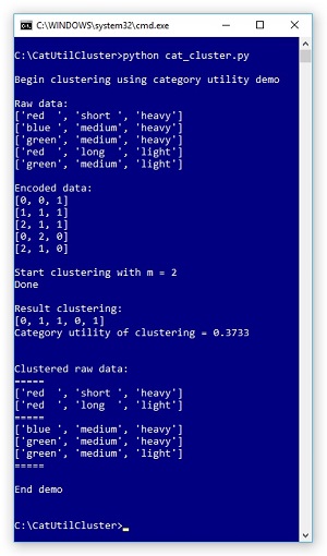
Take a look at the screenshot of a demo program in Figure 1. The demo clusters the five-item example dataset described above. Behind the scenes, the dataset is encoded so that each string value, like "red," is represented by a 0-based integer index. The demo sets the number of clusters to use, m, as 2. After clustering completed, the result was displayed as [0, 1, 1, 0, 1]. This means item (0) is in cluster 0, item (1) is in cluster 1, item (2) is in cluster 1, item (3) is in cluster 0, and item (4) is in cluster 1.
In terms of the raw data, the resulting clustering is:
k=0
(0)  red    short   heavy
(3)  red    long    light

k=1
(1)  blue   medium  heavy
(2)  green  medium  heavy
(4)  green  medium  light
The CU value of this clustering is 0.3733 which, as it turns out, is the best possible CU for this dataset. If you look at the result clustering, you should get an intuitive notion that the clustering makes sense.
This article assumes you have intermediate or better programming skill with a C-family language but doesn't assume you know anything about clustering or category utility.
The demo is coded in Python, the language of choice for machine learning. But you shouldn't have too much trouble refactoring the code to another language if you wish. The entire source code for the demo is presented in this article, and the code is also available in the accompanying download.
Understanding Category Utility
The CU of a given clustering of a dataset is a numeric value that reflects how good the clustering is. Larger values of CU indicate a better clustering. If you have a goodness-of-clustering metric such as CU, then clustering can be accomplished in several ways. For example, in pseudo-code, one way to cluster a dataset ds into m clusters is:
initialize m clusters with one item each
loop each remaining item
  compute CU values if item placed in each cluster
  assign item to cluster that gives largest CU
end-loop
This is called a greedy agglomerative technique because each decision is based on the current best CU value (greedy) and the clustering is built up one item at a time (agglomerative).
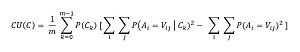
The math definition of CU is shown in Figure 2. The equation looks intimidating but is simpler than it appears. The calculation is best explained by example.
 [Click on image for larger view.]
Figure 2. Math Equation for Category Utility
[Click on image for larger view.]
Figure 2. Math Equation for Category Utility
In the equation, C is a clustering, A is an attribute, such as "color," and V is a value, such as "red". The equation has two summation terms. The right-most summation for the demo dataset is calculated as:
red:    (2/5)^2 = 0.160
blue    (1/5)^2 = 0.040
green:  (2/5)^2 = 0.160

short:  (1/5)^2 = 0.040
medium: (3/5)^2 = 0.360
long:   (1/5)^2 = 0.040

light:  (2/5)^2 = 0.160
heavy:  (3/5)^2 = 0.360

sum =             1.320
This sum is an indirect representation of how well you could do by guessing values without any clustering. For example, for an unknown item, if you guessed the color is "red," your probability of being correct is 2/5.
The left-hand summation is similar except that you look at each cluster separately. For k = 0:
red:    (2/2)^2 = 1.000
blue    (0/2)^2 = 0.000
green:  (0/2)^2 = 0.000

short:  (1/2)^2 = 0.250
medium: (0/2)^2 = 0.000
long:   (1/2)^2 = 0.250

light:  (1/2)^2 = 0.250
heavy:  (1/2)^2 = 0.250

sum =             2.000
And then for k = 1:
red:    (0/3)^2 = 0.000
blue    (1/3)^2 = 0.111
green:  (2/3)^2 = 0.444

short:  (0/3)^2 = 0.000
medium: (3/3)^2 = 1.000
long:   (0/3)^2 = 0.000

light:  (1/3)^2 = 0.111
heavy:  (2/3)^2 = 0.444

sum =             2.111
These sums are also indirect measures of how well you could do by guessing values, but this time conditioned with clustering information.
The P(Ck) values mean, "probability of cluster k." Because cluster k = 0 has 2 items and cluster k = 1 has 3 items, the two P(C) values are 2/5 = 0.40 and 3/5 = 0.60 respectively. The P(Ck) values adjust for cluster size. The 1/m term is a scaling factor that takes the number of clusters into account.
The last step when calculating CU is to put the terms together according to the definition:
CU = 1/2 * (0.40 * (2.000 - 1.320) + 0.60 * (2.111 - 1.320))
   = 0.3733
A CU value is a measure of how much information you gain by a clustering. Larger values of CU mean you've gained more information, and therefore larger CU values mean better clustering. Very clever! Ideas similar to CU have been around for decades, but to the best of my knowledge, the definition I use was first described in a 1985 research paper by M. Gluck and J. Corter.
The Demo Program
To create the demo program, I used Notepad. The demo code was written using the Anaconda 4.1.1 distribution (Python 3.5.2 and NumPy 1.14.0), but there are no significant dependencies so any Python 3x and NumPy 1x versions should work.
The overall structure of the program is:
# cat_cluster.py
import numpy as np

def cat_utility(ds, clustering, m): . . .
def cluster(ds, m): . . .
def main():
  print("Begin clustering demo ")
  . . .
  print("End demo ")

if __name__ == "__main__":
  main()
I removed all normal error checking, and I indented with two spaces instead of the usual four, to save space.
Program-defined function cat_utility() computes the CU of a encoded dataset ds, based on a clustering, with m clusters. Function cluster() performs a greedy agglomerative clustering using the cat_utility() function.
All the control logic is contained in a function main(). The function begins by setting up that source data to be clustered:
raw_data = [['red  ', 'short ', 'heavy'],
            ['blue ', 'medium', 'heavy'],
            ['green', 'medium', 'heavy'],
            ['red  ', 'long  ', 'light'],
            ['green', 'medium', 'light']]
I decided to use a list instead of a NumPy array-of-arrays style matrix. In a non-demo scenario you'd read raw data into memory from a text file. Although it's not apparent, the demo program assumes your data has been set up so that the first m items are different because these items will act as the first items in each cluster.
Next, the demo sets up encoded data:
enc_data = [[0, 0, 1],
            [1, 1, 1],
            [2, 1, 1],
            [0, 2, 0],
            [2, 1, 0]]
In a non-demo scenario you'd want to encode data programmatically, or possibly encode by dropping the raw data into Excel and then doing replace operations on each column.
Next, the raw and encoded data are displayed like so:
print("Raw data: ")
for item in raw_data:
  print(item)

print("Encoded data: ")
for item in enc_data:
  print(item)
Clustering is performed by these statements:
m = 2
print("Start clustering m = %d " % m)
clustering = cluster(enc_data, m)
print("Done")
print("Result clustering: ")
print(clustering)
Almost all clustering techniques, for both numeric and non-numeric data, require you to specify the number of clusters to use. After clustering, the CU of the result clustering is computed and displayed:
cu = cat_utility(enc_data, clustering, m)
print("CU of clustering %0.4f \n" % cu)
The demo concludes by displaying the raw data in clustered form:
print("Clustered raw data: ")
print("=====")
for k in range(m):
  for i in range(len(enc_data)):
    if clustering[i] == k:
      print(raw_data[i])
  print("=====")
Computing Category Utility
The code for function cat_utility() is presented in Listing 1. The logic follows the example calculation by hand I explained previously. Most of the code sets up all the various counts of data items.
Listing 1. The cat_utility() Function
def cat_utility(ds, clustering, m):
  # category utility of clustering of dataset ds
  n = len(ds)  # number items
  d = len(ds[0])  # number attributes/dimensions

  cluster_cts = [0] * m  # [0,0]
  for ni in range(n):  # each item
    k = clustering[ni]
    cluster_cts[k] += 1

  for i in range(m):
    if cluster_cts[i] == 0:   # cluster no items
      return 0.0

  unique_vals = [0] * d  # [0,0,0]
  for i in range(d):  # each att/dim
    maxi = 0
    for ni in range(n):  # each item
      if ds[ni][i] > maxi: maxi = ds[ni][i]
    unique_vals[i] = maxi+1

  att_cts = []
  for i in range(d): # each att
    cts = [0] * unique_vals[i]
    for ni in range(n):  # each data item
      v = ds[ni][i]
      cts[v] += 1
    att_cts.append(cts)

  k_cts = []
  for k in range(m):  # each cluster
    a_cts = []
    for i in range(d): # each att
      cts = [0] * unique_vals[i]
      for ni in range(n):  # each data item
        if clustering[ni] != k: continue
        v = ds[ni][i]
        cts[v] += 1
      a_cts.append(cts)
    k_cts.append(a_cts)

  un_sum_sq = 0.0
  for i in range(d):
    for j in range(len(att_cts[i])):
      un_sum_sq += (1.0 * att_cts[i][j] / n) \
      * (1.0 * att_cts[i][j] / n)

  cond_sum_sq = [0.0] * m
  for k in range(m):  # each cluster
    sum = 0.0
    for i in range(d):
      for j in range(len(att_cts[i])):
        if cluster_cts[k] == 0:
          print("FATAL LOGIC ERROR")
        sum += (1.0 * k_cts[k][i][j] / cluster_cts[k]) \
        * (1.0 * k_cts[k][i][j] / cluster_cts[k])
    cond_sum_sq[k] = sum

  prob_c = [0.0] * m  # [0.0, 0.0]
  for k in range(m):  # each cluster
    prob_c[k] = (1.0 * cluster_cts[k]) / n

  left = 1.0 / m
  right = 0.0
  for k in range(m):
    right += prob_c[k] * (cond_sum_sq[k] - un_sum_sq)
  cu = left * right
  return cu
The function begins by determining the number of items to cluster and the number of attributes in the dataset:
n = len(ds)  # number items
d = len(ds[0])  # number attributes/dimensions
Because these values don't change, they can be calculated just once and passed to the function as parameters, at the expense of a more complex interface.
The function computes the number to items assigned to each cluster. If any cluster has no items assigned, the function returns 0.0 which indicates a worst-possible clustering:
for i in range(m):
  if cluster_cts[i] == 0: # cluster has no items
    return 0.0
An alternative is to return a special error value such as -1.0 or throw an exception. The right-hand unconditional sum of squared probabilities term is calculated like so:
un_sum_sq = 0.0
for i in range(d):
  for j in range(len(att_cts[i])):
    un_sum_sq += (1.0 * att_cts[i][j] / n) \
    * (1.0 * att_cts[i][j] / n)
Here att_cts[i][j] is a list-of-lists where [i] indicates the attribute (0, 1, 2) for (color, length, weight) and [j] indicates the value, for example (0, 1, 2) for (red, blue, green). The indexing is quite tricky but you can think of function cat_utility() as a black box because you won't have to modify the code except in rare scenarios.
Using Category Utility for Clustering
At first thought, you might think that you could repeatedly try random clusterings, keep track of their CU values, and then use the clustering that gave the best CU value. Unfortunately, the number of possible clusterings for all but tiny datasets is unimaginably large. For example, the demo has n = 5 and k = 2 and there are 15 possible clusterings. But for n = 100 and k = 20, there are approximately 20^100 possible clusterings which is about 1.0e+130 which is a number far greater than the estimated number of atoms in the visible universe!
The code for function cluster() is presented in Listing 2. The most important part of the function, and the code you may want to modify, is the initialization:
working_set = [0] * m
for k in range(m):
  working_set[k] = list(ds[k])

clustering = list(range(m))
The clustering process starts with a copy of the first m items from the dataset. The initial clustering is [0, 1, . . m-1] so the first items are assigned to different clusters. This means that it's critically important that the dataset be preprocessed in some way so that the first m items are as different as feasible.
Listing 2. The cluster() Function
def cluster(ds, m):
  n = len(ds)  # number items to cluster
  working_set = [0] * m
  for k in range(m):
    working_set[k] = list(ds[k])

  clustering = list(range(m))

  for i in range(m, n):
    item_to_cluster = ds[i]
    working_set.append(item_to_cluster)

    proposed_clusterings = []
    for k in range(m):         # proposed
      copy_of_clustering = list(clustering)
      copy_of_clustering.append(k)
      proposed_clusterings.append(copy_of_clustering)

    proposed_cus = [0.0] * m
    for k in range(m):
      proposed_cus[k] = \
        cat_utility(working_set,
          proposed_clusterings[k], m)

    best_proposed = np.argmax(proposed_cus)
    clustering.append(best_proposed)
  return clustering
Instead of preprocessing, an alternative approach is to programmatically randomize, but doing so is surprisingly tricky. Data preprocessing is a key task in most machine learning scenarios.
The loop that performs the clustering agglomeration is:
for i in range(m, n):
  item_to_cluster = ds[i]
  working_set.append(item_to_cluster)
  # consruct k proposed new clusterings
  # compute CU of each proposed
  # assign item to best option
The demo code processes each of the non-initial data items in order. You should either preprocess the source data so that the items are in a random order, or you can programmatically walk through the dataset in a random order.
The demo code uses a pure greedy strategy. An alternative is to use what's called epsilon-greedy. Instead of always selecting the best alternative (the option that gives the largest CU value), you can select a random item with a small probability. This approach also inserts some randomness into the clustering process.
Wrapping Up
Data clustering is an NP-hard problem. Loosely, this means there is no way to find an optimal clustering without examining every possible clustering. Therefore, the demo code is not guaranteed to find the best clustering.
One way to increase the likelihood of an optimal clustering is to cluster several times with different initial cluster assignments and using different orders when processing the data. You can programmatically keep track of which initialization and order sequence gives the best result (largest CU value) and use that result.
The technique presented in this article can be used to cluster mixed numeric and non-numeric data. The idea is to convert numeric data into non-numeric data by binning. For example, if data items represent people and one of the data attributes is age, you could bin ages 1 through 10 as "very young," ages 11 through 20 as "teen" and so on.
About the Author
Dr. James McCaffrey directs the data science and research efforts at Quaetrix, a data analytics company located near Redmond, Washington. Before joining Quaetrix, James was a senior research engineer at Microsoft. James can be reached at [email protected].