The Data Science Lab
Neural Regression Using Keras
The goal of a regression problem is to make a prediction of a numeric value. For example, you might want to predict the price of a house based on its square footage, age, ZIP code and so on. Regression problems require a different set of techniques than classification problems where the goal is to predict a categorical value such as the color of a house.
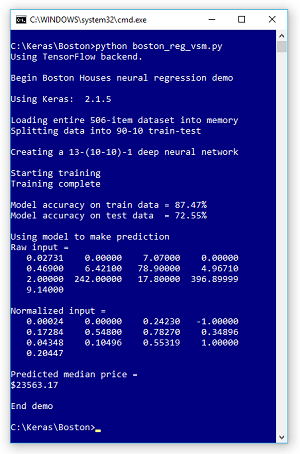
In this article I'll demonstrate how to perform regression using a deep neural network with the Keras code library. The best way to understand where this article is headed is to take a look at the screenshot of a demo program in Figure 1.
The demo program creates a prediction model on the Boston Housing dataset where the goal is to predict the median house price in one of 506 towns close to Boston. The demo loads the 506 data items into memory and then randomly splits the data into a training dataset (90 percent = 455 items) and a test dataset (10 percent = the remaining 51 items).
The demo creates a 13-(10-10)-1 neural network. There are 13 predictor values such as crime index of the town, average number of rooms per house in the town and so on. There is one output value because the goal is to predict a single numeric value. The neural network has two hidden processing layers, each of which has 10 nodes. The number of input and output nodes is determined by your data, but the number of hidden layers and the number of nodes in each is a free parameter that must be determined by trial and error.
The demo trains the neural network -- that is, the weights and biases that define the behavior of the neural network are computed using the training data that has known correct input and output values. After training, the demo computes the accuracy of the model on the training data (87.47 percent) and on the test data that was held out during training (72.55 percent). The test accuracy is a rough measure of how well you'd expect the model to do on new, previously unseen data.
The demo concludes by making a prediction for one of the 506 towns. The 13 raw input values are (0.02731, . . 9.14). When the neural regression model was trained, normalized data (scaled so all values are between 0.0 and 1.0) was used, so when making a prediction the demo had to use normalized data which is (0.00024, . . 0.20447). The model predicts the median house price is $23,563.17 which is quite close to the actual median price of $21,600.
 [Click on image for larger view.]
Figure 1. Neural Regression using Keras Demo Run
[Click on image for larger view.]
Figure 1. Neural Regression using Keras Demo Run
This article assumes you have intermediate or better programming skill with a C-family language and a basic familiarity with machine learning. The complete demo code is presented in this article. The source code and the data file used by the demo are also available in the download that accompanies this article. All normal error checking has been removed to keep the main ideas as clear as possible.
Installing Keras
Keras is a code library that provides a relatively easy-to-use Python language interface to the relatively difficult-to-use TensorFlow library. Installing Keras involves three main steps. First you install Python and several required auxiliary packages such as NumPy and SciPy, then you install TensorFlow, then you install Keras.
Although it's possible to install Python and the packages required to run Keras separately, it's much better to install a Python distribution. For my demo, I installed the Anaconda3 4.1.1 distribution (which contains Python 3.5.2), TensorFlow 1.7.0 and Keras 2.1.5.
Understanding the Data
The Boston Housing dataset comes from a research paper written in 1978 that studied air pollution. You can find different versions of the dataset in many locations on the Internet. I used the data at https://archive.ics.uci.edu/ml/machine-learning-databases/housing/. The first data item is:
0.00632, 18.00, 2.310, 0, 0.5380, 6.5750, 65.20,
4.0900, 1, 296.0, 15.30, 396.90, 4.98, 24.00
Each data item has 14 values and represents one of 506 towns near Boston. The first 13 numbers are the values of predictor variables and the last value is the median house price in the town (divided by 1,000). Briefly, the 13 predictor variables are: crime rate in the town, large lot percentage, industry information, Charles River information, pollution, average number rooms per house, house age information, distance to Boston, accessibility to highways, tax rate, pupil-teacher ratio, proportion of Black residents and percentage of low-status residents.
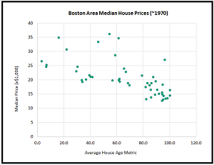
Because there are 14 variables, it's not possible to visualize the dataset, but you can get a rough idea of the data from the graph in Figure 2. The graph shows median house price as a function of the house-age variable, for the first 50 items in the dataset.
 [Click on image for larger view.]
Figure 2. Median House Price as a Function of the House-Age Variable
[Click on image for larger view.]
Figure 2. Median House Price as a Function of the House-Age Variable
The house-age variable, by itself, cannot make a good prediction of the median house price. For example, if you knew the house-age value for a town was 60.0, the median house price could be anything between $18,000 and $36,000 (note that house prices were much lower in the 1970s than they are today).
In most scenarios, it's advisable to normalize your data so that values with large magnitudes, such as a pupil-teacher ratio of 20.0, don't overwhelm small values, such as a pollution reading of 0.538. I used min-max normalization on the 13 predictor variables. For each variable, I computed the min value and the max value, and then for every value x, normalized as (x - min) / (max - min). After min-max normalization, all values will be between 0.0 and 1.0.
The median house values in the raw data were already normalized by dividing by 1,000, so the values ranged from 5.0 to 50.0 with most about 25.0. I applied an additional normalization by dividing the prices by 10 so that all median house prices were between 0.5 and 5.0 with most being around 2.5.
The Demo Program
The structure of demo program, with a few minor edits to save space, is presented in Listing 1. I indent two spaces rather than the usual four spaces to save space. And note that Python uses the "\" character for line continuation. I used Notepad to edit my program but many of my colleagues prefer Visual Studio or VS Code, both of which have excellent support for Python.
Listing 1: The Boston Housing Demo Program Structure
# boston_reg_vsm.py

import numpy as np
import keras as K
import os
os.environ['TF_CPP_MIN_LOG_LEVEL']='2'

def my_print(arr, wid, cols, dec): . . .
def my_accuracy(model, data_x, data_y,
  pct_close): . . .

def main():
  print("Begin demo ")
  np.random.seed(1)
  kv = K.__version__
  print("Using Keras: ", kv, "\n")

  # load all data into memory
  # split data into train-test sets
  # define a 13-(10-10)-1 neural net
  # train the neural net
  # compute accuracy on train and test data
  # use trained model to make a predction

  print("End demo ")

if __name__=="__main__":
  main()
The file is named boston_reg_vsm.py where the "vsm" stands for Visual Studio Magazine. For simplicity, the demo imports the entire Keras library. An alternative is to import just the modules or functions needed. The os package is used just to suppress an annoying startup message.
The demo defines two helper functions. Function my_print() displays an array arr using wid width, in cols values per row, using dec decimals. Function my_accuracy() is important. When training a neural regression model there is no built-in definition of the accuracy of a prediction. You must define how close a predicted value must be to a target value in order to be counted as a correct prediction.
All the control logic for the demo program is contained in a single main() function. Program execution begins by setting the global numpy random seed so results will be reproducible. The demo prints out the version of Keras being used. In a non-demo scenario you should document or display the versions of all libraries used (Python, NumPy, TensorFlow and so on) because new versions are released frequently.
Custom Accuracy and Print
The definitions for program-defined helper functions my_print() and my_accuracy() are shown in Listing 2. The print function is optional, and I wrote it just to give a pretty output.
Listing 2: Program-Defined Helper Functions
def my_print(arr, wid, cols, dec):
  fmt = "% " + str(wid) + "." + str(dec) + "f "
  for i in range(len(arr)):
    if i > 0 and i % cols == 0: print("")
    print(fmt % arr[i], end="")
  print("")

def my_accuracy(model, data_x, data_y, pct_close):
  correct = 0; wrong = 0
  n = len(data_x)
  for i in range(n):
    predicted = model.predict(np.array([data_x[i]],
      dtype=np.float32) )  # [[ x ]]
    actual = data_y[i]
    if np.abs(predicted[0][0] - actual) < \
      np.abs(pct_close * actual):
      correct += 1
    else:
      wrong += 1
  return (correct * 100.0) / (correct + wrong)
Function my_accuracy() walks through each item in data_x, which is a two-dimensional matrix, and sends the item to the built-in predict() function. The result is compared to the correct result stored in data_y. If the computed result is within pct_close of the target result, the prediction is counted as correct. For example, if pct_close = 0.10 and predicted = 3.50 and actual = 3.00 the prediction would be marked as wrong. Only predictions between 2.70 and 3.30 would be counted as correct. The function returns accuracy as a percentage between 0 and 100 as opposed to a proportion between 0 and 1.
Loading Data into Memory
The demo loads data in memory using the NumPy loadtxt() function:
print("Loading entire 506-item dataset into memory")
data_file = ".\\Data\\boston_mm_tab.txt"
all_data = np.loadtxt(data_file, delimiter="\t",
  skiprows=0, dtype=np.float32)
The code assumes that the data is located in a subdirectory named Data. The loadtxt() function has a lot of optional parameters. In this case, the function call specifies that the data is tab-delimited and that there isn't a header row to skip.
The demo splits the 506 items into training and test sets. The first step is to scramble the order of the data items and then peel off the predictor x-values and the median house price y-values into intermediate matrices like so:
print("Splitting data into 90-10 train-test")
n = len(all_data)  # number rows
indices = np.arange(n)  # an array [0, 1, . . 505]
np.random.shuffle(indices)     # by ref
ntr = int(0.90 * n)  # number training items
data_x = all_data[indices,:-1]  # all rows, skip last col
data_y = all_data[indices,-1]  # all rows, just last col
The shuffle() function operates on its array argument by reference so you don't have to capture a return value. The syntax for NumPy array and matrix indexing is a bit tricky but the comments should give you enough information to modify the code if necessary. The second step is to divide the two intermediate matrices into training and test sets:
train_x = data_x[0:ntr,:]  # rows 0 to ntr-1, all cols
train_y = data_y[0:ntr]    # items 0 to ntr-1
test_x = data_x[ntr:n,:]
test_y = data_y[ntr:n]
Data wrangling isn't conceptually difficult, but it's almost always quite time-consuming and annoying. Many of my colleagues like to use the pandas (originally "panel data," now "Python data analysis library") package to manipulate data, but pandas has a hard learning curve.
Creating the Neural Network
The demo prepares to create the 13-(10-10)-1 neural network with these statements:
my_init = K.initializers.RandomUniform(minval=-0.01,
  maxval=0.01, seed=1)
simple_sgd = K.optimizers.SGD(lr=0.010)
model = K.models.Sequential()
An initializer object with evenly distributed random values between -0.01 and +0.01 is generated, with a seed value of 1 so that the neural net will be reproducible. Neural networks are often highly sensitive to initializations so when things go wrong, this is one of the first areas to investigate.
A basic stochastic gradient descent object is created with a learning rate set to 0.01. The learning rate is a hyperparameter and its value must be determined by trial and error. The neural network object is implicitly created by a call to the Sequential() method. The terms neural network and model are technically different but are typically used interchangeably. Some of my colleagues prefer to use the term "neural network" before training and use the term "model" after training.
The neural network is created like so:
model.add(K.layers.Dense(units=10, input_dim=13,
  activation='tanh', kernel_initializer=my_init))
model.add(K.layers.Dense(units=10,
  activation='tanh', kernel_initializer=my_init))
model.add(K.layers.Dense(units=1, activation=None,
  kernel_initializer=my_init))
model.compile(loss='mean_squared_error',
  optimizer=simple_sgd, metrics=['mse'])
The first hidden layer accepts 13 input values, uses hyperbolic tangent activation, and the uniform random initializer. The second hidden layer is similar, but it accepts the 10 values from the first hidden layer (the input dimension is implicit). Because the network has more than one hidden layer, it is called a deep neural network. The output layer has a single output node with no activation -- this is the design pattern to use for regression problems.
The model object is compiled (to TensorFlow) using mean squared error. Although there are alternatives to mean squared error for a regression neural network, they are rarely used.
Training the Model
Once a neural network has been created, it is very easy to train using Keras:
print("Starting training")
max_epochs = 1000
h = model.fit(train_x, train_y, batch_size=1,
  epochs=max_epochs, verbose=0)  # use 1 or 2
print("Training complete")
One epoch in Keras is defined as touching all training items one time. The number of epochs to use is a hyperparameter. The demo uses a batch size of 1, which is called online training. A more common approach is to use a batch size like 8 or 16, which is called mini-batch training. Deep neural networks can be sensitive to the batch size, so when training fails, this is one of the first hyperparameters to adjust.
The verbose flag controls how much information is displayed during training. The demo sets verbose=0, which suppresses all output. In a non-demo scenario you definitely want to see messages so you identify when training has stalled as quickly as possible. It is possible to create a custom class to perform logging, but that's a topic outside the scope of this article.
The Keras fit() function has a lot of parameters. Luckily most have sensible default values. Two of the parameters I often use are initial_epoch and validation_data. You can set initial_epoch to start training in situations where you had to halt training for some reason. You can use validation_data to evaluate error/loss to determine when model overfitting is starting to occur. The demo captures the return object from fit(), which is a log of training history information, but doesn't use it.
The demo program doesn't save the trained model but in most cases you'll want to do so. For example:
mp = ".\\Models\\boston_reg_model.h5"
model.save(mp)
This code would save the model using the default hierarchical data format, which you can think of as sort of like a binary XML. It is also possible to save check-point models during training using the custom callback mechanism.
Evaluating and Using the Trained Model
After training completes, the demo program evaluates the prediction accuracy of the model on the training and test datasets:
acc = my_accuracy(model, train_x, train_y, 0.15)
print("Model accuracy on train data = %0.2f%%" % acc)
acc = my_accuracy(model, test_x, test_y, 0.15)
print("Model accuracy on test data  = %0.2f%%" % acc)
As I mentioned earlier, there's no inherent notion of prediction accuracy for regression problems. The demo counts a prediction as correct if it is within 15 percent of the true median house price.
The demo doesn't display the model loss/error but could have done so like this:
train_mse = model.evaluate(train_x, train_y, verbose=0)
test_mse = model.evaluate(test_x, test_y, verbose=0)
print(train_mse[0])
print(test_mse[0])
In most situations the whole point of training a regression model is to use it to make a prediction. The demo program makes a prediction using the second data item from the original 506 items:
raw_inpt = np.array([[0.02731, 0.00, 7.070, 0, 0.4690,
  6.4210, 78.90, 4.9671, 2, 242.0, 17.80, 396.90,
  9.14]], dtype=np.float32)

norm_inpt = np.array([[0.000236, 0.000000, 0.242302,
  -1.000000, 0.172840, 0.547998, 0.782698, 0.348962,
  0.043478, 0.104962, 0.553191, 1.000000, 0.204470]],
  dtype=np.float32)
When you have new data, you must remember to normalize the predictor values in the same way that the training data was normalized. For min-max normalization that means you need to save the min and max value for every variable that was normalized.
The demo echoes the input using the program-defined my_print() function:
print("Using model to make prediction")
print("Raw input = ")
my_print(raw_inpt[0], 10, 4, 5)
print("Normalized input =")
my_print(norm_inpt[0], 10, 4, 5)
The demo concludes by making and displaying the prediction:
. . .
  med_price = model.predict(norm_inpt)
  med_price[0,0] *= 10000
  print("\nPredicted median price = ")
  print("$%0.2f" % med_price[0,0])
  print("\nEnd demo ")
if __name__=="__main__":
  main()
The predicted value is returned as a 1x1 matrix so [0,0] holds the actual value. Recall that the original median house prices were normalized by dividing by 1,000 but the demo divided by an additional factor of 10, therefore to get the original, unnormalized predicted median house price, you must multiply by 10,000.