The Data Science Lab
Q-Learning Using Python
Reinforcement learning (RL) is a branch of machine learning that addresses problems where there is no explicit training data. Q-learning is an algorithm that can be used to solve some types of RL problems. In this article I demonstrate how Q-learning can solve a maze problem.
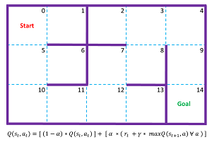
The best way to see where this article is headed is to take a look at the image of a simple maze in Figure 1 and a screenshot of an associated demo program in Figure 2. The 3x5 maze has 15 cells, numbered from 0 to 14. The goal is to get from cell 0 in the upper left corner, to cell 14 in the lower right corner, in the fewest moves. You can move left, right, up, or down but not diagonally.
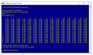
The demo program sets up a representation of the maze in memory and then uses a Q-learning algorithm to find a Q matrix. The Q stands for quality, where larger values are better. The row indices are the "from" cells and the column indices are the "to" cells. If the starting cell is 0, then scanning that row shows the largest Q value is 0.02 at to-cell 5. Then at cell 5, the largest value in the row is 0.05 at to-cell 10. The process continues until the program reaches the goal state at cell 14.
It's not likely your boss at work will ask you to write Q-learning code to solve a maze, but this problem is the "Hello World" for Q-learning because the problem is easy to understand and visualize.
 [Click on image for larger view.]
Figure 1. Simple Maze Problem
[Click on image for larger view.]
Figure 1. Simple Maze Problem
 [Click on image for larger view.]
Figure 2. Q-Learning Demo Program
[Click on image for larger view.]
Figure 2. Q-Learning Demo Program
This article assumes you have intermediate or better programming skill but doesn't assume you know anything about Q-learning. The demo program is coded using Python, but you shouldn't have too much trouble refactoring the code to another language, such as C# or JavaScript. All the code for the demo program is presented in this article, and it's also available in the accompanying file download.
Straight to the Code
In my opinion, Q-learning is best understood by first looking at the code. The overall structure of the demo program, with a few minor edits to save space, is presented in Listing 1.
Listing 1: Q-Learning Demo Program Structure
# maze.py
import numpy as np

# =============================================================

def my_print(Q, dec): . . .
def get_poss_next_states(s, F, ns): . . .
def get_rnd_next_state(s, F, ns): . . .
def train(F, R, Q, gamma, lrn_rate, goal, ns, max_epochs): . .
def walk(start, goal, Q): . . .

# =============================================================

def main():
  np.random.seed(1)
  print("Setting up maze in memory")

  F = np.zeros(shape=[15,15], dtype=np.int)  # Feasible
  F[0,1] = 1; F[0,5] = 1; F[1,0] = 1; F[2,3] = 1; F[3,2] = 1
  F[3,4] = 1; F[3,8] = 1; F[4,3] = 1; F[4,9] = 1; F[5,0] = 1
  F[5,6] = 1; F[5,10] = 1; F[6,5] = 1; F[7,8] = 1; F[7,12] = 1
  F[8,3] = 1; F[8,7] = 1; F[9,4] = 1; F[9,14] = 1; F[10,5] = 1
  F[10,11] = 1; F[11,10] = 1; F[11,12] = 1; F[12,7] = 1;
  F[12,11] = 1; F[12,13] = 1; F[13,12] = 1; F[14,14] = 1

  R = np.zeros(shape=[15,15], dtype=np.int)  # Rewards
  R[0,1] = -0.1; R[0,5] = -0.1; R[1,0] = -0.1; R[2,3] = -0.1
  R[3,2] = -0.1; R[3,4] = -0.1; R[3,8] = -0.1; R[4,3] = -0.1
  R[4,9] = -0.1; R[5,0] = -0.1; R[5,6] = -0.1; R[5,10] = -0.1
  R[6,5] = -0.1; R[7,8] = -0.1; R[7,12] = -0.1; R[8,3] = -0.1
  R[8,7] = -0.1; R[9,4] = -0.1; R[9,14] = 10.0; R[10,5] = -0.1
  R[10,11] = -0.1; R[11,10] = -0.1; R[11,12] = -0.1
  R[12,7] = -0.1; R[12,11] = -0.1; R[12,13] = -0.1
  R[13,12] = -0.1; R[14,14] = -0.1

# =============================================================

  Q = np.zeros(shape=[15,15], dtype=np.float32)  # Quality

  print("Analyzing maze with RL Q-learning")
  start = 0; goal = 14
  ns = 15  # number of states
  gamma = 0.5
  lrn_rate = 0.5
  max_epochs = 1000
  train(F, R, Q, gamma, lrn_rate, goal, ns, max_epochs)
  print("Done ")

  print("The Q matrix is: \n ")
  my_print(Q, 2)

  print("Using Q to go from 0 to goal (14)")
  walk(start, goal, Q)

if __name__ == "__main__":
  main()
I used Notepad as my editor. The main() function begins by setting up an F matrix which defines the feasibility of moving from one cell/state to another. For example, F[7][12] = 1 means you can transition from cell/state 7 to cell/state 12, and F[6][7] = 0 means you cannot move from cell 7 to cell 8 (because there's a wall in the way).
The R matrix defines a reward for moving from one cell to another. Most feasible moves give a negative reward of -0.1, which punishes moves that don't make progress and therefore discourages going in circles. The one big reward is R[9][14] = 10.0, which moves you to the goal state.
Most of the work is done by the train() function, which computes the values of the Q matrix. Q-learning is iterative, so a maximum number of iterations, 1,000, is set. Q-learning has two parameters, the learning rate and gamma. Larger values of the learning rate increase the influence of both current rewards and future rewards (explore) at the expense of past rewards (exploit). The value of gamma, also called the discount factor, influences the importance of future rewards. These values must be determined by trial and error but using 0.5 is typically a good starting place.
After the Q matrix has been computed, function walk() uses the matrix to display the shortest path through the maze: 0->5->10->11->12->7->8->3->4->9->14->done.
The Helper Functions
The train() function uses two helpers, get_poss_next_states() and get_rnd_next_state(). Function get_poss_next_states() is defined:
def get_poss_next_states(s, F, ns):
  poss_next_states = []
  for j in range(ns):
    if F[s,j] == 1: poss_next_states.append(j)
  return poss_next_states
For a given cell state s, the function uses the F matrix to determine which states can be reached, and returns those states as a list. For example, if s = 5, the return list is [0, 6, 10].
Function get_rnd_next_state() is defined:
def get_rnd_next_state(s, F, ns):
  poss_next_states = get_poss_next_states(s, F, ns)
  next_state = \
    poss_next_states[np.random.randint(0,\
    len(poss_next_states))]
  return next_state
For a given state s, all possible next states are determined, and then one of those states is randomly selected. For example, if s = 5, the candidates are [0, 6, 10]. The call to np.randomint() returns a random value from 0 to 2, which acts as the index into the candidate list.
Computing the Q Matrix
The heart of the demo program is function train(), which computes the Q matrix. The code for train() is presented in Listing 2. The Q-learning update equation, shown at the bottom of Figure 1, is based on a clever idea called the Bellman equation. You don't need to understand the Bellman equation to use Q-learning, but if you're interested, the Wikipedia article on the Bellman equation is a good place to start.
Listing 2: The train() Function
def train(F, R, Q, gamma, lrn_rate, goal, ns, max_epochs):
  for i in range(0,max_epochs):
    curr_s = np.random.randint(0,ns)  # random start state

    while(True):
      next_s = get_rnd_next_state(curr_s, F, ns)
      poss_next_next_states = \
        get_poss_next_states(next_s, F, ns)

      max_Q = -9999.99
      for j in range(len(poss_next_next_states)):
        nn_s = poss_next_next_states[j]
        q = Q[next_s,nn_s]
        if q > max_Q:
          max_Q = q
      # Q = [(1-a) * Q]  +  [a * (rt + (g * maxQ))]
      Q[curr_s][next_s] = ((1 - lrn_rate) * Q[curr_s] \
        [next_s]) + (lrn_rate * (R[curr_s][next_s] + \
        (gamma * max_Q)))

      curr_s = next_s
      if curr_s == goal: break
In words, you repeatedly start at a random state in the maze. Then, at each cell position, you pick a random next state and you also determine all possible states after the next state -- these are sometimes called "next-next states." You examine the current Q values and find the largest value from the next state to any next-next state. This largest value, max_Q, is used in the statement that updates the Q matrix.
For each random starting state, you repeat this process until you reach the goal state. This assumes the goal state is reachable, so in some problems you need to apply a maximum loop control variable.
For example, suppose at some point during training, you're at cell 4 and the next random state is selected as cell 9. The next-next states are 4 and 14. Because moving to cell 14 has a reward of +10.0, the value of Q[4][9] will be increased, making that path more attractive than the path from cell 4 to cell 3. Clever!
Walking the Q Matrix
After the Q matrix has been computed, it can be used by function walk() to show the shortest path from any starting cell to any goal cell in the maze. Function walk() is defined:
def walk(start, goal, Q):
  curr = start
  print(str(curr) + "->", end="")
  while curr != goal:
    next = np.argmax(Q[curr])
    print(str(next) + "->", end="")
    curr = next
  print("done")
The key to function walk() is function np.argmax(), which returns the index of the largest value of the function's input vector. For example, if a vector v had values (8, 6, 9, 4, 5, 7), then a call to np.argmax(v) would return 2. Function walk() assumes the goal state is reachable.
The demo program defines a helper method my_print() to display a computed Q matrix:
def my_print(Q):
  rows = len(Q); cols = len(Q[0])
  print("       0      1      2      3      4      5\
      6      7      8      9      10     11     12\
     13     14")
  for i in range(rows):
    print("%d " % i, end="")
    if i < 10: print(" ", end="")
    for j in range(cols): print(" %6.2f" % Q[i,j], end="")
    print("")
  print("")
Function my_print() is a hard-coded hack designed to work only with the demo maze.
Wrapping Up
The Q-learning example presented here should give you a reasonably solid understanding of the general principles involved. The main problem scenario is one where you have a set of discrete states, and the challenge is to perform a sequence of actions that finds a long-term reward, without explicitly defining rules. Q-learning can be useful when you can safely train a physical system with many trials, such as training a vacuum cleaning robot how to navigate through a room. But Q-learning isn't applicable in scenarios like training a driverless car how to navigate through traffic (unless you have a very sophisticated simulation system available).
About the Author
Dr. James McCaffrey works for Microsoft Research in Redmond, Wash. He has worked on several Microsoft products including Azure and Bing. James can be reached at jamccaff@microsoft.com.