The Data Science Lab
Neural Anomaly Detection Using Keras
An advantage of using a neural technique compared to a standard clustering technique is that neural techniques can handle non-numeric data by encoding that data.
Anomaly detection, also called outlier detection, is the process of finding rare items in a dataset. Examples include finding fraudulent login events and fake news items.
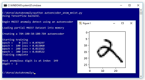
Take a look at the demo program in Figure 1. The demo examines a 1,000-item subset of the well-known MNIST (modified National Institute of Standards and Technology) dataset. Each item is a 28 x 28 grayscale image (784 pixels) of a handwritten digit from "0'" to "9".
 [Click on image for larger view.]
Figure 1. Anomaly Detection on the MNIST Dataset
[Click on image for larger view.]
Figure 1. Anomaly Detection on the MNIST Dataset
The demo program creates and trains a 784-100-50-100-784 deep neural autoencoder using the Keras library. An autoencoder is a neural network that learns to predict its input. After training, the demo scans through the 1,000 images and finds the one image which is most anomalous, where most anomalous means highest reconstruction error. The most anomalous digit is a "2" that looks like it could be a "9" digit or a script lowercase "a" character.
This article assumes you have intermediate or better programming skill with a C-family language and a basic familiarity with machine learning but doesn't assume you know anything about autoencoders. All the demo code and the data file are presented in this article. They're also available in the download that accompanies this article. All normal error checking has been removed to keep the main ideas as clear as possible.
Installing Keras
Keras is a code library that provides a relatively easy-to-use Python language interface to the relatively difficult-to-use TensorFlow library. Installing Keras involves two main steps. First you install Python and several required auxiliary packages such as NumPy and SciPy. Then you install TensorFlow and Keras as add-on Python packages.
Although it's possible to install Python and the packages required to run Keras separately, it's much better to install a Python distribution, which is a collection containing the base Python interpreter and additional packages that are compatible with each other. For my demo, I installed the Anaconda3 5.2.0 distribution (which contains Python 3.6.5).
After installing Anaconda, I used the pip utility to install TensorFlow 1.11.0, and then I used pip to install Keras 2.2.4. The demo program has no significant Python or Keras dependencies, so any relatively recent versions will work. Note that when you install TensorFlow, you get an embedded version of Keras, but most of my colleagues and I prefer to use separate TensorFlow and Keras packages.
The Demo Program
The structure of demo program, with a few minor edits to save space, is presented in Listing 1. I indent with two spaces rather than the usual four spaces to save space. Note that Python uses the "\" character for line continuation. I used Notepad to edit my program. Most of my colleagues prefer a more sophisticated editor, but I like the enforced simplicity of Notepad.
Listing 1: The Anomaly Detection Demo Program Structure
# autoencoder_anom_mnist.py
# anomaly detection for the MNIST digits

import numpy as np
import keras as K
import matplotlib.pyplot as plt
import os
os.environ['TF_CPP_MIN_LOG_LEVEL']='2'  # suppress CPU msg

def display(raw_data_x, raw_data_y, idx):
  label = raw_data_y[idx]  # like '5'
  print("digit = ", str(label), "\n")
  pixels = np.array(raw_data_x[idx])  # target row of pixels
  pixels = pixels.reshape((28,28))
  plt.rcParams['toolbar'] = 'None'
  plt.imshow(pixels, cmap=plt.get_cmap('gray_r'))
  plt.show()

# -----------------------------------------------------------

class MyLogger(K.callbacks.Callback):
  def __init__(self, n):
    self.n = n   # print loss every n epochs

  def on_epoch_end(self, epoch, logs={}):
    if epoch % self.n == 0:
      curr_loss =logs.get('loss')
      print("epoch = %4d loss = %0.6f" % (epoch, curr_loss))

def main():
  # 0. get started
  print("Begin MNIST anomaly detect using an autoencoder ")
  np.random.seed(1)  # not used

  # 1. load data into memory
  # 2. define autoencoder model
  # 3. compile model
  # 4. train model
  # 5. save model
  # 6. use model to find anomaly

if __name__=="__main__":
  main()
The demo program starts by importing the NumPy, Keras, OS and Matplotlib packages. Notice you don't need to explicitly import TensorFlow. The OS package is used just to suppress an annoying startup message. The Matplotlib package is used to visually display the most anomalous digit that's found by the model.
Loading Data into Memory
Working with the raw MNIST data is a bit difficult because it's saved in a binary and proprietary format. I wrote a utility program to extract the first 1,000 items from the 60,000 training items. I saved the data as mnist_keras_1000.txt in a Data subdirectory.
The resulting data looks like:
7 ** 0 255 67 . . 123
2 ** 113 28 0 . . 206
. . .
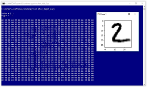
Each line represents one digit. The first value on each line is the digit. The second value is an arbitrary double asterisk sequence just for readability. The next 28 x 28 = 784 values are grayscale pixel values between 0 and 255. All values are separated by a single blank space character. Figure 2 shows the data item at index [1] in the data file, which is a typical "2" digit.
 [Click on image for larger view.]
Figure 2. A Typical MNIST Digit
[Click on image for larger view.]
Figure 2. A Typical MNIST Digit
The data is loaded into memory with these statements:
# 1. load data
print("Loading Keras version MNIST data into memory \n")
data_file = ".\\Data\\mnist_keras_1000.txt"
data_x = np.loadtxt(data_file, delimiter=" ",
  usecols=range(2,786), dtype=np.float32)
labels = np.loadtxt(data_file, delimiter=" ",
  usecols=[0], dtype=np.float32)
norm_x = data_x / 255
Notice the digit-label is in column 0 and the 784 pixel values are in columns 2 to 785. After all 1,000 images are loaded into memory, a normalized version of the data is created by dividing each pixel value by 255 so that the normalized pixel values are all between 0.0 and 1.0.
Defining the Autoencoder Model
The demo program creates and compiles a deep autoencoder model with the code shown in Listing 2. The number of input values and output values (784) are determined by the data but the number of hidden layers and the number of nodes in each hidden layer, are free parameters (also called hyperparameters) that must be determined by trial and error.
Similarly, the weight initialization algorithm (Glorot uniform) and the hidden layer activation function (tanh) and the output layer activation function (tanh) are hyperparameters. Because all input and output values are between 0.0 and 1.0 for this problem, logistic sigmoid is a strong alternative for output activation.
The model is compiled using the Adam optimization algorithm which usually gives better results than the simpler stochastic gradient descent algorithm.
Listing 2: Creating and Compiling the Autoencoder Model
# 2. define autoencoder model
print("Creating a 784-100-50-100-784 autoencoder ")
my_init = K.initializers.glorot_uniform(seed=1)
autoenc = K.models.Sequential()
autoenc.add(K.layers.Dense(input_dim=784, units=100,
  activation='tanh', kernel_initializer=my_init))
autoenc.add(K.layers.Dense(units=50,
  activation='tanh', kernel_initializer=my_init))
autoenc.add(K.layers.Dense(units=100,
  activation='tanh', kernel_initializer=my_init))
autoenc.add(K.layers.Dense(units=784,
  activation='tanh', kernel_initializer=my_init))

# 3. compile model
simple_adam = K.optimizers.adam()
autoenc.compile(loss='mean_squared_error',
  optimizer=simple_adam)
The model uses mean squared error for the training loss function because an autoencoder is essentially a regression problem rather than a classification problem,
Training and Evaluating the Autoencoder Model
The model is trained with these statements:
# 4. train model
print("Starting training")
max_epochs = 400
my_logger = MyLogger(n=100)
h = autoenc.fit(norm_x, norm_x, batch_size=40,
  epochs=max_epochs, verbose=0, callbacks=[my_logger])
print("Training complete")

# 5. save model
# TODO
The maximum number of training epochs is a hyperparameter. The program-defined MyLogger object displays the current training loss mean squared error every 100 epochs so you can monitor progress. The batch size, 40, is another hyperparameter. Notice that the fit() function uses the norm_x data for both input and output values. The label data is used only for visualization.
After training, you'll usually want to save the model but that's a bit outside the scope of this article. The Keras documentation has several good examples that show how to save a trained model.
When working with autoencoders, in most situations (including this example) there's no inherent definition of model accuracy. You must determine how close computed output values must be to the associated input values in order to be counted as a correct prediction, and then write a program-defined function to compute your metric.
Using the Autoencoder Model to Find Anomalous Data
After autoencoder model has been trained, the idea is to find data items that are difficult to correctly predict, or equivalently, difficult to reconstruct. The demo code scans through all 1,000 data items and calculates the squared difference between the normalized input values and the computed output values like this:
# 6. find most anomalous data item
N = len(norm_x)
max_se = 0.0; max_ix = 0
predicteds = autoenc.predict(norm_x)
for i in range(N):
  diff = norm_x[i] - predicteds[i]
  curr_se = np.sum(diff * diff)
  if curr_se > max_se:
    max_se = curr_se; max_ix = i
The maximum squared error is calculated and the index of the associated image is saved. An alternative to finding the single item with the largest reconstruction error is to save all squared errors, sort them and return the top-n items where the value of n will depend on the particular problem you're investigating.
After the most anomalous data item has been found, it is shown using the program-defined display() function:
raw_data_x = data_x.astype(np.int)
raw_data_y = labels.astype(np.int)
print("Most anomalous digit is at index ", max_ix)
display(raw_data_x, raw_data_y, max_ix)
The pixel and label values are converted from type float32 to int mostly as a matter of principle because the Matplotlib imshow() function can accept either data type.
Wrapping Up
Anomaly detection using a deep neural autoencoder is not a well-known technique. An advantage of using a neural technique compared to a standard clustering technique is that neural techniques can handle non-numeric data by encoding that data. Most clustering techniques depend on a distance measure which means the source data must be strictly numeric.
A related, but also little-explored, technique for anomaly detection is to create an autoencoder for the dataset under investigation. Then, instead of using reconstruction error to find anomalous data, you can cluster the data because the inner-most hidden layer nodes hold a strictly numeric representation of each data item. After clustering, you can look for clusters that have very few data items, or look for data items within clusters that are most distant from their cluster centroid.
About the Author
Dr. James McCaffrey works for Microsoft Research in Redmond, Wash. He has worked on several Microsoft products including Azure and Bing. James can be reached at [email protected].