The Data Science Lab
Weighted k-NN Classification Using Python
The weighted k-nearest neighbors (k-NN) classification algorithm is a relatively simple technique to predict the class of an item based on two or more numeric predictor variables. For example, you might want to predict the political party affiliation (democrat, republican, independent) of a person based on their age, annual income, gender, years of education and so on. In this article I explain how to implement the weighted k-nearest neighbors algorithm using Python.
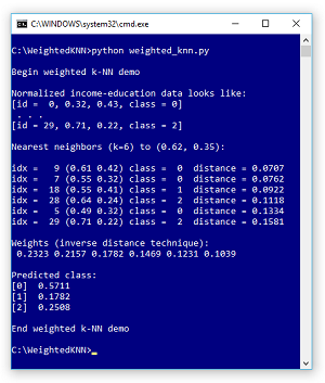
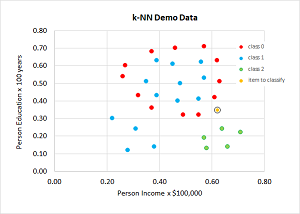
Take a look at the screenshot of a demo run in Figure 1 and a graph of the associated data in Figure 2. The demo program sets up 30 dummy data items. Each item represents a person's income, education level and a class to predict (0, 1, 2). The data has only two predictor variables so it can be displayed in a graph, but k-NN works with any number of predictors.
The demo data has been normalized so all values are between 0.0 and 1.0. When using k-NN, it's important to normalize the data so that large values don't overwhelm small values. The goal of the demo is to predict the class of a new person who has normalized income and education of (0.62, 0.35). The demo sets k = 6 and finds the six labeled data items that are closet to the item-to-classify.
 [Click on image for larger view.]
Figure 1. Weighted k-NN Classification Demo Run
[Click on image for larger view.]
Figure 1. Weighted k-NN Classification Demo Run
After identifying the six closet labeled data items, the demo uses a weighted voting technique to reach a decision. The weighted voting values for classes (0, 1, 2) are (0.5711, 0.1782, 0.2508) so an item at (0.62, 0.35) would be predicted as class 0.
 [Click on image for larger view.]
Figure 2. Weighted k-NN Data
[Click on image for larger view.]
Figure 2. Weighted k-NN Data
This article assumes you have intermediate or better programming skill with Python or a C-family language but doesn't assume you know anything about the weighted k-NN algorithm. The complete demo code and the associated data are presented in this article.
How the Weighted k-NN Algorithm Works
When using k-NN you must compute the distances from the item-to-classify to all the labeled data. Using the Euclidean distance is simple and effective. The Euclidean distance between two items is the square root of the sum of the squared differences of coordinates. For example, if a labeled data item is (0.40, 0.70) and the item to classify is (0.55, 0.60) then:
dist = sqrt( (0.40 - 0.55)^2 + (0.70 - 0.60)^2 )
       = sqrt(0.0225 + 0.0100)
       = 0.1803
After computing all distances and finding the k-nearest distances, you must use a voting algorithm to determine the predicted class. The demo program uses the inverse weights technique, which is best explained by example. Suppose, as in the demo, the six closet distances are (0.0707, 0.0762, 0.0922, 0.1118, 0.1334, 0.1581) and the associated labeled classes are (0, 0, 1, 2, 0, 2).
You compute the inverse of each distance, find the sum of the inverses, then divide each inverse by the sum. For the demo, the inverses are (14.1443, 13.1234, 10.8460, 8.9445, 7.4963, 6.3251). The sum of the inverses is 60.8796. Dividing each inverse distance by the sum gives the weights: (0.2323, 0.2157, 0.1782, 0.1469, 0.1231, 0.1039).
Each weight is a vote for its associated class. In the demo, the first, second and fifth closest items have class 0, so the vote for class 0 is the sum of the first, second and fifth weights: 0.2323 + 0.2157 + 0.1231 = 0.5711. Similarly, the vote for class 1 is 0.1782 and the vote for class 2 is 0.1469 + 0.1039 = 0.2508. The predicted class is the one with the greatest vote, class 0 in this case.
The Demo Program
The complete demo program, with a few minor edits to save space, is presented in Listing 1. I used Notepad to edit my program but many of my colleagues prefer Visual Studio Code, which has excellent support for Python. I indent with two spaces instead of the usual four to save space.
Listing 1: The Weighted k-NN Demo Program
# k_nn.py
# k nearest neighbors demo
# Anaconda3 5.2.0 (Python 3.6.5)

import numpy as np

def dist_func(item, data_point):
  sum = 0.0
  for i in range(2):
    diff = item[i] - data_point[i+1]
    sum += diff * diff
  return np.sqrt(sum)

def make_weights(k, distances):
  result = np.zeros(k, dtype=np.float32)
  sum = 0.0
  for i in range(k):
    result[i] += 1.0 / distances[i]
    sum += result[i]
  result /= sum
  return result

def show(v):
  print("idx = %3d (%3.2f %3.2f) class = %2d  " \
    % (v[0], v[1], v[2], v[3]), end="")

def main():
  print("\nBegin weighted k-NN demo \n")
  print("Normalized income-education data looks like: ")
  print("[id =  0, 0.32, 0.43, class = 0]")
  print(" . . . ")
  print("[id = 29, 0.71, 0.22, class = 2]")

  data = np.array([
    [0, 0.32, 0.43, 0], [1, 0.26, 0.54, 0],
    [2, 0.27, 0.60, 0], [3, 0.37, 0.36, 0],
    [4, 0.37, 0.68, 0], [5, 0.49, 0.32, 0],
    [6, 0.46, 0.70, 0], [7, 0.55, 0.32, 0],
    [8, 0.57, 0.71, 0], [9, 0.61, 0.42, 0],
    [10, 0.63, 0.51, 0], [11, 0.62, 0.63, 0],
    [12, 0.39, 0.43, 1], [13, 0.35, 0.51, 1],
    [14, 0.39, 0.63, 1], [15, 0.47, 0.40, 1],
    [16, 0.48, 0.50, 1], [17, 0.45, 0.61, 1],
    [18, 0.55, 0.41, 1], [19, 0.57, 0.53, 1],
    [20, 0.56, 0.62, 1], [21, 0.28, 0.12, 1],
    [22, 0.31, 0.24, 1], [23, 0.22, 0.30, 1],
    [24, 0.38, 0.14, 1], [25, 0.58, 0.13, 2],
    [26, 0.57, 0.19, 2], [27, 0.66, 0.14, 2],
    [28, 0.64, 0.24, 2], [29, 0.71, 0.22, 2]],
    dtype=np.float32)

  item = np.array([0.62, 0.35], dtype=np.float32)
  print("\nNearest neighbors (k=6) to (0.62, 0.35): ")

  # 1. compute all distances to item
  N = len(data)
  k = 6
  c = 3
  distances = np.zeros(N)
  for i in range(N):
    distances[i] = dist_func(item, data[i])

  # 2. get ordering of distances
  ordering = distances.argsort()

  # 3. get and show info for k nearest
  k_near_dists = np.zeros(k, dtype=np.float32)
  for i in range(k):
    idx = ordering[i]
    show(data[idx])  # pretty formatting
    print("distance = %0.4f" % distances[idx])
    k_near_dists[i] = distances[idx]  # save dists

  # 4. vote
  votes = np.zeros(c, dtype=np.float32)
  wts = make_weights(k, k_near_dists)
  print("\nWeights (inverse distance technique): ")
  for i in range(len(wts)):
    print("%7.4f" % wts[i], end="")

  print("\n\nPredicted class: ")
  for i in range(k):
    idx = ordering[i]
    pred_class = np.int(data[idx][3])
    votes[pred_class] += wts[i] * 1.0
  for i in range(c):
    print("[%d]  %0.4f" % (i, votes[i]))

  print("\nEnd weighted k-NN demo ")

if __name__ == "__main__":
  main()
The demo program uses a static code approach rather than an OOP approach for simplicity. All normal error-checking has been omitted.
Loading Data into Memory
The demo program hard-codes the dummy data and the item-to-classify:
data = np.array([
  [0, 0.32, 0.43, 0],
  # etc.
  [29, 0.71, 0.22, 2]],
  dtype=np.float32)
item = np.array([0.62, 0.35], dtype=np.float32)
In a non-demo scenario you'd likely store your data in a text file and load it into a NumPy array-of-arrays matrix using the loadtxt() function. The first value in each data item is an arbitrary ID. I used consecutive integers from 0 to 29, but the k-NN algorithm doesn't need data IDs so the ID column could have been omitted. The second and third values are the normalized predictor values. The fourth value is the class ID. Class IDs for k-NN don't need to be zero-based integers, but using this scheme is programmatically convenient.
Computing Distances
The first step in the k-NN algorithm is to compute the distance from each labeled data item to the item-to-be classified. The demo implementation of Euclidean distance is:
def dist_func(item, data_point):
  sum = 0.0
  for i in range(2):
    diff = item[i] - data_point[i+1]
    sum += diff * diff
  return np.sqrt(sum)
Notice that the for-loop indexing is hard-coded with 2 for the number of predictor values, and the difference between item[i] and data_point[i+1] is offset to account for the data ID value at position [0]. There's usually a tradeoff between coding a machine learning algorithm for a specific problem and coding the algorithm with a view towards general purpose use. Because k-NN is so simple and easy to implement, I usually use the code-for-specific problem approach.
Sorting or Ordering the Distances
After all distances have been computed, the k-NN algorithm must find the k-nearest (smallest) distances. One approach is to augment the entire labeled dataset with each distance value, then explicitly sort the augmented data. An alternative approach, used by the demo, is to use a neat NumPy argsort() function that returns the order of data if it were to be sorted. For example, if an array named distances held values (0.40, 0.30, 0.10, 0.90, 0.50) then distances.argsort() returns (2, 1, 0, 4, 3).
Determining k-NN Weights and Voting
The most primitive form of using the k-nearest distances to predict a class is to use a simple majority rule approach. For example, if k = 4 and c = 3, and two of the closet distances are associated with class 2, and one closest distance is associated with class 0, and one closest distance is associated with class 1, then a majority rule approach predicts class 2. Note that weighted k-NN using uniform weights, each with value 1/k, is equivalent to the majority rule approach.
The majority rule approach has two significant problems, First, ties are possible. Second, all distances are equally weighted. The most common weighting scheme for weighted k-NN is to apply the inverse weights approach used by the demo program. Another approach is to use the rank of the k-nearest distances (1, 2, . . 6) instead of the distances themselves. For k = 6 this rank order centroid weights would be calculated as (1 + 1/2 + 1/3 + 1/4 + 1/5 + 1/6) / 6 = 0.4083, (1/2 + 1/3 + 1/4 + 1/5 + 1/6) / 6 = 0.2417 and so on.
Wrapping Up
The weighted k-NN classification algorithm has received increased attention recently for two reasons. First, by using neural autoencoding, k-NN can deal with mixed numeric and non-numeric predictor values. Second, compared to many other classification algorithms, notably neural networks, the results of weighted k-NN are relatively easy to interpret. Interpretability has become increasingly important due to legal requirements of machine learning techniques from laws such as the European Union's GDPR.
About the Author
Dr. James McCaffrey works for Microsoft Research in Redmond, Wash. He has worked on several Microsoft products including Azure and Bing. James can be reached at [email protected].