The Data Science Lab
How to Do Naive Bayes with Numeric Data Using C#
Dr. James McCaffrey of Microsoft Research uses a full code sample and screenshots to demonstrate how to create a naive Bayes classification system when the predictor values are numeric, using the C# language without any special code libraries.
The Naive Bayes technique can be used for binary classification, for example predicting if a person is male or female based on predictors such as age, height, weight, and so on), or for multiclass classification, for example predicting if a person is politically conservative, moderate or liberal based on predictors such as annual income, sex, and so on. Naive Bayes classification can be used with numeric predictor values, such as a height of 5.75 feet, or with categorical predictor values such as a height of "tall".
In this article I explain how to create a naive Bayes classification system when the predictor values are numeric, using the C# language without any special code libraries. A good way to see where this article is headed is to take a look at the screenshot of a demo program in Figure 1.
 [Click on image for larger view.]
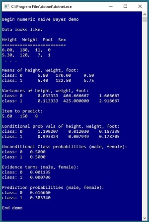
Figure 1. Naive Bayes Classification with Numeric Data
[Click on image for larger view.]
Figure 1. Naive Bayes Classification with Numeric Data
The goal of the demo program is to predict the gender of a person (male = 0, female = 1) based on their height, weight, and foot length. Behind the scenes, the demo program sets up eight reference items. Next the demo computes the mean and variance for each of the three predictor variables, for each of the two classes to predict. Then the demo sets up a new data item to classify, with predictor values of height = 5.60, weight = 150, foot = 8.
Using the mean and variance information, the demo computes conditional probability values, unconditional class probabilities, and what are called evidence terms. The evidence terms are used to compute the prediction probabilities for each of the two classes. For the demo data, the probability that the unknown item is male is about 0.62 and the probability of female is 0.38, therefore the conclusion is the unknown person is most likely male.
This article assumes you have intermediate or better skill with C# but doesn’t assume you know anything about naive Bayes classification. The complete code for the demo program shown in Figure 1 is presented in this article. The code is also available in the file download that accompanies this article.
The Demo Program
To create the demo program, I launched Visual Studio 2019. I used the Community (free) edition but any relatively recent version of Visual Studio will work fine. From the main Visual Studio start window I selected the “Create a new project” option. Next, I selected C# from the Language dropdown control and Console from the Project Type dropdown, and then picked the “Console App (.NET Core)” item.
The code presented in this article will run as a .NET Core console application or as a .NET Framework application. Many of the newer Microsoft technologies, such as the ML.NET code library, specifically target .NET Core so it makes sense to develop most C# machine learning code in that environment.
I entered “NumericBayes” as the Project Name, specified C:\VSM on my local machine as the Location (you can use any convenient directory), and checked the “Place solution and project in the same directory” box.
After the template code loaded into Visual Studio, at the top of the editor window I removed all using statements to unneeded namespaces, leaving just the reference to the top level System namespace. The demo needs no other assemblies and uses no external code libraries.
In the Solution Explorer window, I renamed file Program.cs to the more descriptive NumericBayesProgram.cs and then in the editor window I renamed class Program to class NumericBayesProgram to match the file name. The structure of the demo program, with a few minor edits to save space, is shown in Listing 1.
Listing 1. Numeric Bayes Demo Program Structure
using System;
namespace NumericBayes
{
  class NumericBayesProgram
  {
    static void Main(string[] args)
    {
      Console.WriteLine("Begin naive Bayes demo");

      Console.WriteLine("Data looks like: ");
      Console.WriteLine("Height Weight Foot Sex");
      Console.WriteLine("======================");
      Console.WriteLine("6.00,  180,  11,  0");
      Console.WriteLine("5.30,  120,   7,  1");
      Console.WriteLine(" . . .");

      double[][] data = new double[8][];
      data[0] = new double[] { 6.00, 180, 11, 0 };
      data[1] = new double[] { 5.90, 190,  9, 0 };
      data[2] = new double[] { 5.70, 170,  8, 0 };
      data[3] = new double[] { 5.60, 140, 10, 0 };

      data[4] = new double[] { 5.80, 120, 9, 1 };
      data[5] = new double[] { 5.50, 150, 6, 1 };
      data[6] = new double[] { 5.30, 120, 7, 1 };
      data[7] = new double[] { 5.00, 100, 5, 1 };

      int N = data.Length;  // 8 items

      // compute class counts
      // compute and display means
      // compute and display variances
      // set up item to predict
      // compute and display conditional probs
      // compute and display unconditional probs
      // compute and display evidence terms
      // compute and display prediction probs

      Console.WriteLine("End demo");
      Console.ReadLine();
    } // Main

    static double ProbDensFunc(double u, double v,
      double x)
    {
      double left =
        1.0 / Math.Sqrt(2 * Math.PI * v);
      double right =
        Math.Exp(-(x-u) * (x-u) / (2*v));
      return left * right;
    }
  } // Program class
} // ns
All of the program logic is contained in the Main method. The demo uses a helper function ProbDensFunc() that computes the probability density function value of a point x for a Gaussian distribution with mean u and variance v.
 [Click on image for larger view.]
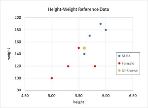
Figure 2. Partial Graph of the Demo Reference Data
[Click on image for larger view.]
Figure 2. Partial Graph of the Demo Reference Data
The reference data that is used to determine the class of an unknown data item is hard-coded into an array-of-arrays style matrix. In a non-demo scenario you'd probably use a helper function named something like MatLoad() to read data from a text file into a matrix.
Because the reference data has three predictor variables -- height, weight, foot -- the data can't be visualized in a two-dimensional graph. But you can get a good idea of the structure of the data by examining the partial graph of just height and weight in Figure 2. The reference data is not linearly separable, meaning that there is no straight line or hyperplane that can divide the data so that all instance of one class are on one side of the line/plane and all instances of the other class are on the other side. Naive Bayes classification can handle such data in many, but not all, problem scenarios.
The demo program performs binary classification. Although you can use any encoding scheme you wish for the class to predict, using (0, 1) is most convenient because those values will nicely map to vector indices. The technique presented in this article can be easily extended to multiclass classification problems. For example, if the goal was to classify a person as politically conservative, moderate, or liberal, you could encode those three values as 0, 1, or 2 respectively. Note that it's not useful to encode the class label to predict using one-hot encoding, such as you'd do when using a neural network.
Preparing the Prediction
There are four steps to prepare a naive Bayes prediction for numeric data. You must compute the counts of each class to predict, the means of each predictor, the variances of each predictor, and set up the item to predict. The class counts are computed like so:
int N = data.Length;  // 8 items
int[] classCts = new int[2];  // male, female
for (int i = 0; i < N; ++i)
{
  int c = (int)data[i][3];  // class is at [3]
  ++classCts[c];
}
Array classCts holds the number of reference items of each class, 4 male and 4 female in the demo reference data. The count of males is stored at index [0] and the count of females is stored at index [1]. Throughout the demo program I use hard-coded constants such as 2 for the number of classes to predict. In a non-demo scenario you could set up class-scope variables such as:
static int NUMCLASSES = 2;
static int NUMPREDICTORS = 3;
static int NUMITEMS = 8;
The means of each predictor variable, for each class, are computed starting with this code that sums the values of each predictor:
double[][] means = new double[2][];
for (int c = 0; c < 2; ++c)
  means[c] = new double[3];

for (int i = 0; i < N; ++i)
{
  int c = (int)data[i][3];
  for (int j = 0; j < 3; ++j)  // ht, wt, foot
    means[c][j] += data[i][j];
}
The values are stored in an array-of-arrays matrix named means where the first index indicates which class (0 = male, 1 = male) and the second index indicates which predictor (0 = height, 1 = weight, 2 = foot). This design is arbitrary and you could reverse the meaning of the indices if you wish. After the sums of the predictors are computed, they're converted to means by dividing by the number of items in each class:
for (int c = 0; c < 2; ++c)
{
  for (int j = 0; j < 3; ++j)
    means[c][j] /= classCts[c];
}
Although it's not strictly necessary, the demo program displays the values of the means:
Console.WriteLine("Means of height, weight, foot:");
for (int c = 0; c < 2; ++c)
{
  Console.Write("class: " + c + "  ");
  for (int j = 0; j < 3; ++j)
    Console.Write(means[c][j].
      ToString("F2").PadLeft(8) + " ");
  Console.WriteLine("");
}
Displaying intermediate values is a good way to catch errors early. For example, it's easy to manually calculate the mean of the heights of males: (6.00 + 5.90 + 5.70 + 5.60) / 4 = 5.80 and verify your program has computed the means correctly.
The statistical sample variance of a set of n values with a mean of u is sum[(x – u)^2] / (n – 1). For example, if there are three values = (1, 4, 10) then u = 5.0 and the variance is (1 – 5.0)^2 + (4 – 5.0)^ (10 – 5.0)^2 / (3 – 1) = (16 + 1 + 25) / 2 = 21.00. The demo sets up storage for the variances of each predictor using the same indexing scheme that's used for the means:
double[][] variances = new double[2][];
for (int c = 0; c < 2; ++c)
  variances[c] = new double[3];
Next, the demo sums the squared differences for each predictor:
for (int i = 0; i < N; ++i)
{
  int c = (int)data[i][3];
  for (int j = 0; j < 3; ++j)
  {
    double x = data[i][j];
    double u = means[c][j];
    variances[c][j] += (x - u) * (x - u);
  }
}
Then the sums are divided by one less than each class count to get the sample variances:
for (int c = 0; c < 2; ++c)
{
  for (int j = 0; j < 3; ++j)
    variances[c][j] /= classCts[c] - 1;
}
The computed variances of each predictor are displayed by this code:
Console.WriteLine("Variances of ht, wt, foot:");
for (int c = 0; c < 2; ++c)
{
  Console.Write("class: " + c + "  ");
  for (int j = 0; j < 3; ++j)
    Console.Write(variances[c][j].
      ToString("F6").PadLeft(12));
  Console.WriteLine("");
}
The last of the four steps of the preparation phase is to set up the item to predict:
double[] unk = new double[] { 5.60, 150, 8 };
Console.WriteLine("Item to predict:");
Console.WriteLine("5.60   150   8");
Unlike some machine learning techniques such as logistic regression where you use training data to create a general prediction model that can be applied to any new data item, in naive Bayes you use reference data and an item to predict to essentially create a new model for each prediction.
Making the Prediction
To make a prediction, you use the item to predict, the means, and the variances to compute conditional probabilities. An example of a conditional probability is P(height = 5.70 | C = 0) which is read, "the probability that the height is 5.70 given that the class is 0."
Storage for the conditional probabilities uses the same indexing scheme that is used for means and variances, where the first index indicate the class and the second index indicates the predictor:
double[][] condProbs = new double[2][];
for (int c = 0; c < 2; ++c)
  condProbs[c] = new double[3];
The conditional probabilities are computed using the ProbDensFunc() helper function:
for (int c = 0; c < 2; ++c)  // each class
{
  for (int j = 0; j < 3; ++j)  // each predictor
  {
    double u = means[c][j];
    double v = variances[c][j];
    double x = unk[j];
    condProbs[c][j] = ProbDensFunc(u, v, x);
  }
}
The probability density function defines the shape of the Gaussian bell-shaped curve. Note that these values really aren't probabilities because they can be greater than 1.0, but they're usually called probabilities anyway.
The conditional probabilities are displayed like so:
Console.WriteLine("Conditional probs:");
for (int c = 0; c < 2; ++c)
{
  Console.Write("class: " + c + "  ");
  for (int j = 0; j < 3; ++j)
    Console.Write(condProbs[c][j].
      ToString("F6").PadLeft(12));
  Console.WriteLine("");
}
Unconditional probabilities of the classes to predict are ordinary probabilities. For example, the P(C = 0) = 0.5000 because four of the eight data items are class 0. The unconditional probabilities are computed and displayed by this code:
double[] classProbs = new double[2];
for (int c = 0; c < 2; ++c)
  classProbs[c] = (classCts[c] * 1.0) / N;

Console.WriteLine("Unconditional probs:");
for (int c = 0; c < 2; ++c)
  Console.WriteLine("class: " + c + "   " +
    classProbs[c].ToString("F4"));
Next, what are called evidence terms for each class are computed. Suppose P(C = 0) = 0.5000, P(height = 5.60 | C = 0) = 1.20, P(weight = 150 | C = 0) = 0.01, P(foot = 8 | C = 0) = 0.16 then the evidence that the class is 0 equals the product of the four terms: 0.5000 * 1.20 * 0.01 * 0.16 = 0.00096. The demo computes the evidence terms for each class with this code:
double[] evidenceTerms = new double[2];
for (int c = 0; c < 2; ++c)
{
  evidenceTerms[c] = classProbs[c];
  for (int j = 0; j < 3; ++j)
    evidenceTerms[c] *= condProbs[c][j];
}
The evidence terms are displayed by these statements:
Console.WriteLine("Evidence terms:");
for (int c = 0; c < 2; ++c)
  Console.WriteLine("class: " + c +
    "   " + evidenceTerms[c].ToString("F6"));
Notice that an evidence term is the product of several values that are usually less than 1.0 so there's a chance of an arithmetic underflow error. In a non-demo scenario you can reduce the likelihood of such an error by using a log trick. For example, x1 * x2 * x3 = exp(log(x1) + log(x2) + log(x3)). Instead of multiplying many small values, you can add the log of each value then apply the exp() function to the sum.
The last step in making a prediction is to convert the evidence terms to probabilities. You compute the sum of all evidence terms then divide each term by the sum:
double sumEvidence = 0.0;
for (int c = 0; c < 2; ++c)
  sumOfEvidences += evidenceTerms[c];

double[] predictProbs = new double[2];
for (int c = 0; c < 2; ++c)
  predictProbs[c] = evidenceTerms[c] / sumEvidence;
The demo program displays the final prediction probabilities with this code:
Console.WriteLine("Prediction probs:");
for (int c = 0; c < 2; ++c)
  Console.WriteLine("class: " + c +
    "   " + predictProbs[c].ToString("F6"));
The predicted class is the one with the largest prediction probability.
Wrapping Up
The naive Bayes classification technique has "naive" in its name because it assumes that each predictor value is mathematically independent. This assumption is often not true. For example a person's height is likely to be strongly correlated with their weight.
Naive Bayes classification with numeric data makes the additional assumption that all predictor variables are Gaussian distributed. Again, this assumption is sometimes not true. For example, the ages of people in a particular profession could be significantly skewed or even bimodal.
In spite of these assumptions, naive Bayes classification often works quite well. Additionally, naive Bayes classification often works well by combining it with a more sophisticated classification technique such as a neural network classifier. Using two or more techniques in this way in machine learning is called an ensemble technique.