The Data Science Lab

Data Prep for Machine Learning: Encoding

Dr. James McCaffrey of Microsoft Research uses a full code program and screenshots to explain how to programmatically encode categorical data for use with a machine learning prediction model such as a neural network classification or regression system.

• By James McCaffrey
• 08/12/2020

This article explains how to programmatically encode categorical data for use with a machine learning (ML) prediction model such as a neural network classification or regression system. Suppose you are trying to predict voting behavior from a file of people data. Your data might include predictor variables like each person's sex (male or female) and region where they live (eastern, western, central), and a dependent variable to predict like political leaning (conservative, moderate, liberal).

Neural networks are essentially complex math functions which work with numeric values. Therefore, categorical predictor variables and categorical dependent variables must be converted to a numeric form. This is called data encoding. There are dozens of types of encoding. The type of encoding to use depends on several factors, including specific ML library being used (such as PyTorch or scikit-learn), and whether a value is a predictor (sometimes called a feature or an independent variable) or a value to predict (sometimes called a class label or a dependent variable).

In situations where your source data file is small, about 500 lines or less, you can usually encode your categorical data manually using a text editor or spreadsheet. But in almost all realistic scenarios with large datasets you must encode data programmatically.

Preparing data for use in an ML system is time consuming, tedious, and error prone. A reasonable rule of thumb is that data preparation requires at least 80 percent of the total time needed to create an ML system. At the large tech company I work for, I oversee a series of 12-week ML projects. It's not uncommon for project teams to spend 11 of the 12 weeks on data preparation and just one week on all other activities combined. There are three main phases of data preparation: cleaning, normalizing and encoding, and splitting. Each of the three phases has several steps.

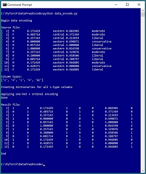
A good way to understand data encoding and see where this article is headed is to take a look at the screenshot of a demo program in Figure 1. The demo uses a small text file named people_normalized.txt where each line represents one person. There are five columns/fields: sex, age, region, income, and political leaning. The data has been processed by removing missing values, editing bad data, and normalizing the numeric age and income values. The sex, region, and political leaning fields must be encoded.

The ultimate goal of a hypothetical ML system is to use the demo data to create a neural network that predicts political leaning from sex, age, region, and income. The demo analyzes the sex and region predictor fields, then encodes those fields using a technique called one-hot encoding. The political leaning field is encoded using ordinal encoding.

The demo is a Python language program but programmatic data encoding can be implemented using any language. The first five lines of the demo source data are:

M  0.171429  eastern 0.802905  moderate
F  0.485714  central 0.371369  moderate
M  0.257143  central 0.213693  liberal
M  0.000000  western 0.690871  conservative
M  0.057143  central 1.000000  liberal
. . .

The demo begins by displaying the source data file. Next, the demo scans through the sex, region, and political leaning columns and constructs a Dictionary object for each of those columns. Then the demo uses the Dictionary objects to compute a one-hot encoding for the sex and region columns, and an ordinal encoding for the political leaning column. For example, "M" is encoded as (1, 0), "central" is encoded as (0, 1, 0), and "liberal" is encoded as 2.

This article assumes you have intermediate or better skill with a C-family programming language. The demo program is coded using Python but you shouldn't have too much trouble refactoring the demo code to another language if you wish. The complete source code for the demo program is presented in this article. The source code is also available in the accompanying file download.

The Data Preparation Pipeline
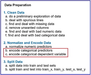
Although data preparation is different for every problem scenario, in general the data preparation pipeline for most ML systems usually follows something similar to the steps shown in Figure 2.

Data preparation for ML is deceptive because the process is conceptually easy. However, there are many steps, and each step is much more complicated than you might expect if you're new to ML. This article explains the eighth and ninth steps in Figure 2. Other Data Science Lab articles explain the other seven steps. The data preparation series of articles can be found here.

The tasks in Figure 2 are usually not followed in a strictly sequential order. You often have to backtrack and jump around to different tasks. But it's a good idea to follow the steps shown in order as much as possible. For example, it's better to normalize data before encoding because encoding generates many additional numeric columns which makes it a bit more complicated to normalize the original numeric data.

Understanding Encoding Techniques
A complete explanation of the many different types of data encoding would literally require an entire book on the subject. But there are a few encoding techniques that are used in the majority of ML problem scenarios. Understanding these few key techniques will allow you to understand the less-common techniques if you encounter them.

In most situations, predictor variables that have three or more possible values are encoded using one-hot encoding, also called 1-of-N or 1-of-C encoding. Suppose you have a predictor variable color which can be one of three values: red, blue, green. You encode red as (1, 0, 0), blue as (0, 1, 0), and green as (0, 0, 1). The ordering of the encoding is arbitrary.

An important alternative encoding technique is called effect coding, also known as 1-of-(N-1) or 1-of-(C-1) encoding. You would encode red as (1, 0), blue as (0, 1), and green as (-1, -1). Another closely related technique is called dummy coding. Dummy coding is often used for classical statistics models but is not used very often for neural-based ML models.

Predictor variables that have just two possible values (binary predictors) are commonly encoded in one of three ways. Suppose you have a predictor variable sex which can be male or female. You can use one-hot encoding: male is encoded as (1, 0) and female is encoded as (0, 1). You can use minus-one-plus-one encoding: male is encoded as -1 and female is encoded as +1. You can use zero-one encoding: male is encoded as 0 and female is encoded as 1.

A dependent variable that has three or more possible values is usually encoded using one-hot encoding or ordinal encoding. If you are trying to predict color, which can be red, blue or green, ordinal encoding is red = 0, blue = 1, green =2.

A dependent variable that has just two possible values is usually encoded using one-hot encoding, or minus-one-plus-one encoding, or zero-one encoding. In many ML scenarios, one specific type of encoding is required. For example, when using the Keras neural network code library, dependent variables with three or more values must be encoded using the one-hot technique. But when using the PyTorch library, dependent variables with three or more values must be encoded using the ordinal encoding technique.

In some ML scenarios, you have a choice of which type of encoding to use. For example, when using the Keras library, you can encode a binary dependent variable using zero-one encoding in conjunction with logistic sigmoid activation, or you can use one-hot encoding in conjunction with softmax activation. When using the PyTorch library, you can encode a binary predictor variable using zero-one encoding in conjunction with one input node, or you can use one-hot encoding in conjunction with two input nodes.

In short, deciding how to encode categorical data for use in an ML system is not trivial. There are many types of encoding. If you are using a code library, you must read the documentation carefully to determine if a specific type of encoding is required.

The Demo Program
The structure of the demo program, with a few minor edits to save space, is shown in Listing 1. I indent my Python programs using two spaces, rather than the more common four spaces or a tab character, as a matter of personal preference. The program has seven worker functions plus a main() function to control program flow. The purpose of worker functions line_count() and show_file() should be clear from their names. Function encode_file() does most of the work. Helper functions make_col_dict(), make_dicts_arr(), one_hot_str(), and ord_str() will be explained when their implementations are presented.

Listing 1: Data Encoding Demo Program

# data_encode.py
# Python 3.7.6  NumPy 1.18.1

import numpy as np

def show_file(fn, start, end, indices=False,
 strip_nl=False): . . . 

def line_count(fn): . . . 

def make_col_dict(data, col, delim): . . .

def make_dicts_arr(fn, col_types,
  delim): . . . 

def one_hot_str(sv, dict, delim): . . .

def ord_str(sv, dict): . . . 

def encode_file(src, dest, col_types,
  dicts_arr, delim): . . . 

def main():
  print("\nBegin data encoding ")

  src = ".\\people_normalized.txt"
  dest = ".\\people_encoded.txt"

  print("\nSource file: ")
  show_file(src, 1, 9999, indices=True,
    strip_nl=True)  

  print("\nColumn types: ")
  col_types = ["c", "n", "c", "n", "dc"] 
  print(col_types)

  print("\nCreating dictionaries for c cols")
  dicts_arr = make_dicts_arr(src,
    col_types, "\t")

  print("\nApply one-hot + ordinal encoding")
  encode_file(src, dest, col_types,
    dicts_arr, "\t")
  print("Done")

  print("\nResult file: ")
  show_file(dest, 1, 9999, indices=True,
    strip_nl=True)

  print("\nEnd \n")

if __name__ == "__main__":
  main()

The execution of the demo program begins with:

def main():
  print("\nBegin data encoding ")
  src = ".\\people_normalized.txt"
  dest = ".\\people_encoded.txt"
  print("\nSource file: ")
  show_file(src, 1, 9999, indices=True,
    strip_nl=True) 
 . . .

The first step when working with any ML data file is to examine the file. The source data is named people_normalized.txt and has only 12 lines to keep the main ideas of data encoding as clear as possible. The number of lines in the file could have been determined by a call to the line_count() function. The entire data file is examined by a call to show_file() with arguments start=1 and end=9999. In most cases with large data files, you'll examine just specified lines of your data file rather than the entire file.

The indices=True argument instructs show_file() to display 1-based line numbers. With some data preparation tasks it's more natural to use 1-based indexing, but with other tasks it's more natural to use 0-based indexing. Either approach is OK but you've got to be careful of off-by-one errors. The strip_nl=True argument instructs function show_file() to remove trailing newlines from the data lines before printing them to the console shell so that there aren't blank lines between data lines in the display.

The demo continues with:

  print("\nColumn types: ")
  col_types = ["c", "n", "c", "n", "dc"] 
  print(col_types)
  print("\nCreating dictionaries for c columns")
  dicts_arr = make_dicts_arr(src, col_types, "\t")
. . .

The demo identifies the type of each column because different types of columns must be normalized and encoded in different ways. There is no standard way to identify columns so you can use whatever scheme is suited to your problem scenario. The demo uses "c" for the two categorical predictor data columns sex and region, "n" for the two numeric predictor columns age and income, and "dc" for the categorical dependent variable column political leaning.

The demo uses program-defined function make_dicts_arr() to compute a dicts_arr array object. The resulting dicts_arr is a NumPy array of references to Dictionary objects, one Dictionary per data column. If a column is not categorical, the corresponding array cell is set to None (roughly equivalent to null in other languages). The categorical columns have a corresponding cell in dicts_arr that is a reference to a Dictionary where the keys are column values like "eastern", "western", "central" and the Dictionary values are a 0-based indexes like 0, 1, 2. For example, for column [0], dicts_arr[0]["M"] is 0 and dicts_arr[0]["F"] is 1. For column [1], dicts_arr[1] is None because column [1] is the age variable, which is numeric.

The demo program concludes with:

. . .
  print("\nApplying one-hot + ordinal encoding")
  encode_file(src, dest, col_types,
    dicts_arr, "\t")
  print("Done")

  print("\nResult file: ")
  show_file(dest, 1, 9999, indices=True,
    strip_nl=True)

  print("\nEnd \n")
if __name__ == "__main__":
  main()

The source file is one-hot encoded on the sex and region columns, and ordinal encoded on the dependent political leaning column. The results are saved to a destination file, and then displayed. As you'll see shortly, you can easily modify encode_file() so that it will use other types of encoding such as zero-one encoding or effect coding.

Examining the Data
When working with data for an ML system you always need to determine how many lines there are in the data, how many columns/fields there are on each line, and what type of delimiter is used. The demo defines a function line_count() as:

def line_count(fn):
  ct = 0
  fin = open(fn, "r")
  for line in fin:
    ct += 1
  fin.close()
  return ct

The file is opened for reading and then traversed using a Python for-in idiom. Each line of the file, including the terminating newline character, is stored into variable named "line" but that variable isn't used. There are many alternative approaches.

The definition of function show_file() is presented in Listing 2. As is the case with all data preparation functions, there are many possible implementations.

Listing 2: Displaying Specified Lines of a File

def show_file(fn, start, end, indices=False,
  strip_nl=False):
  fin = open(fn, "r")

  ln = 1       # advance to start line
  while ln < start:
    fin.readline()
    ln += 1

  while ln <= end:    # show specified lines
    line = fin.readline()
    if line == "": break  # EOF
    if strip_nl == True:
      line = line.strip()
    if indices == True:
      print("[%3d]  " % ln, end="")
    print(line)
    ln += 1
  fin.close()

Because the while-loop terminates with a break statement, if you specify an end parameter value that's greater than the number of lines in the source file, such as 9999 for the 12-line demo data, the display will end after the last line has been printed, which is usually what you want.

Computing Column Ordinal Values
The demo program computes an ordinal integer value for each string value in a categorical column using function make_dicts_arr() which calls helper function make_col_dict(). The make_col_dict() creates a Dictionary object for a single specified 0-based column of a data file. The definition of helper function make_col_dict() is:

def make_col_dict(data, col, delim):
  # make ord dict for one categorical col
  d = dict()
  n = len(data)
  for i in range(n):
    tokens = data[i].split(delim)
    sv = tokens[col]  # string value
    if sv not in d:
      d[sv] = len(d)  # 0, 1, 2, . .
  return d

The function walks through a data object which is an array of strings, where each string is a line of data. Each string is tokenized using the built-in split() function. For example, if the specified column is [2] then the current sv ("string value") is tokens[2] which is "eastern" for the first line of data.

If the current sv is not in the Dictionary object, it is added as the key value, and the current length of the Dictionary object is used as the Dictionary value. For example, if the Dictionary currently holds "eastern" and "western", then d["eastern"] = 0, d["western"] = 1, and the len(d) = 2. If a "central" value is encountered, it is added with len(d) and so d["central"] is 2 and the new len(d) = 3.

Notice that this approach assigns ordinal integers to categorical values based on the order in which they appear in the source data file. In some situations you might want to force a particular set of values like so:

def make_col_7_dict():
  d = dict()
  d["red"] = 0; d["blue"] = 1; d["green"] = 2
  return d

Another approach is to order the source data so that categorical values first appear in the order in which you want ordinal indexes to be assigned. This is a bit hacky and I don't usually use the technique but some of my colleagues do.

The make_col_arr() function accepts a source data file, reads the file into memory as an array of strings, and then calls the make_col_dicts() function on each categorical column, as tagged by the col_types array. The code for make_dicts_arr() is presented in Listing 3.

Listing 3: Creating an Array of Ordinal Indexes Dictionary Objects

def make_dicts_arr(fn, col_types, delim):
  # make an array of dicts for "c", "dc" cols
  num_cols = len(col_types)  # ex:["c", "n", "dc"]
  dict_arr = np.empty(num_cols, dtype=np.object)

  num_lines = line_count(fn)
  data = np.empty(num_lines, dtype=np.object)
  fin = open(fn, "r")
  i = 0
  for line in fin:
    line = line.strip()
    data[i] = line
    i += 1
  fin.close()

  for j in range(num_cols):
    if col_types[j] == "c" or col_types[j] == "dc":
      dict_arr[j] = make_col_dict(data, j, delim)
    else:
      dict_arr[j] = None

  return dict_arr

One of the many minor details when doing programmatic data normalization with Python is that a NumPy array of strings has to be specified as dtype=np.object rather than dtype=np.str as you would expect. The definitions of functions make_dicts_arr() and make_col_dict() point out the idea that data encoding is relatively simple in principle, but encoding in practice is surprisingly tricky because of the many small details that must be attended to.

Encoding the Source File
After an array of Dictionary objects of column ordinal indexes has been created, the demo program uses that array to encode a source file. The definition of function encode_file() is presented in Listing 4. The function opens the source file for reading and a destination file for writing. The source file is processed one line at a time. Each line is split into tokens. Each token is examined and if the token is a categorical column, an encoded vector is computed.

Listing 4: Encoding a Data File

def encode_file(src, dest, col_types,
  dicts_arr, delim):
  # one-hot "c" columns, ord "dc" column
  fin = open(src, "r")
  fout = open(dest, "w")
  for line in fin:
    line = line.strip()  # remove trailing nl
    tokens = line.split(delim)
    if len(col_types) != len(tokens):
      print("FATAL: len(col_types) != len(tokens)")
      input() 

    s = "" 
    for j in range(len(tokens)):  # each column
      if col_types[j] == "c":
        s += one_hot_str(tokens[j], dicts_arr[j],
          delim)
      elif col_types[j] == "dc":
        s += ord_str(tokens[j], dicts_arr[j])
      else:
        s += tokens[j]
     
      if j < len(tokens)-1:  # interior column
        s += "\t"
      else:                  # last column
        s += "\n"
    fout.write(s)
  
  fout.close(); fin.close()
  return

Function encode_file() calls helper functions one_hot_str() and ord_str(). The definition of one_hot_str() is:

def one_hot_str(sv, dict, delim):
  # ex: "red" = "0 tab 1 tab 0"
  n = len(dict)   # num possible values
  v = dict[sv]    # 0 or 1 or 2 or . .
  s = ""
  for i in range(n):
    if i == v: s += "1"
    else: s += "0"
    if i < n-1: s += delim
  return s

The function needs to know the string value (such as "eastern") to encode, the Dictionary of ordinal indexes for the column being encoded, and needs to know how values are to be delimited in the destination file. Similarly, function ord_str() is defined:

def ord_str(sv, dict):
  v = dict[sv]  # 0 or 1 or 2 or . . 
  return str(v)

If you want to use some other form of encoding, such as effect coding or orthogonal encoding, you would define a helper function to do so and then use that helper in the encode_file() function. The approach used by the demo is to encode each categorical value on the fly. An alternative, which is more efficient but slightly more complicated, is to precompute all possible categorical values, store the encodings in a list or as function logic, and then retrieve the precomputed encoded string when needed. For example, you could define:

def encoded_region(region, delim):
  if region == "eastern":
    return "1" + delim + "0" + delim + "0"
  elif region == "western":
    . . .

Because data encoding is usually done just once, simplicity is usually more important than efficiency. There is always a tradeoff between a simple but inflexible implementation versus a more complex but more flexible implementation.

Wrapping Up
The encoding techniques presented in this article handle many, but not all, ML scenarios. A type of ML problem where encoding must be handled very differently is natural language processing (NLP). Suppose you are creating a sentiment analysis system where the input is a movie review paragraph of about 100 words. For such a scenario there would be roughly 20,000 possible English language input words. It would be a bad idea to use one-hot encoding where each input word is encoded as 19,999 zero-values and 1 one-value. For these types of NLP problems you should use what is called a word embedding, which maps each possible word to numeric vector of 100 to 500 floating point values.

• Get Code Download