The Data Science Lab
Binary Classification Using PyTorch: Model Accuracy
In the final article of a four-part series on binary classification using PyTorch, Dr. James McCaffrey of Microsoft Research shows how to evaluate the accuracy of a trained model, save a model to file, and use a model to make predictions.
The goal of a binary classification problem is to predict an output value that can be one of just two possible discrete values, such as "male" or "female." This article is the fourth in a series of four articles that present a complete end-to-end production-quality example of binary classification using a PyTorch neural network. The example problem is to predict if a banknote (think euro or dollar bill) is authentic or a forgery based on four predictor variables extracted from a digital image of the banknote.
The process of creating a PyTorch neural network binary classifier consists of six steps:
- Prepare the training and test data
- Implement a Dataset object to serve up the data
- Design and implement a neural network
- Write code to train the network
- Write code to evaluate the model (the trained network)
- Write code to save and use the model to make predictions for new, previously unseen data
Each of the six steps is fairly complicated, and the six steps are tightly coupled which adds to the difficulty. This article covers the fifth and sixth steps.
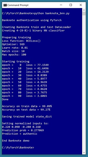
A good way to see where this series of articles is headed is to take a look at the screenshot of the demo program in Figure 1. The demo begins by creating Dataset and DataLoader objects which have been designed to work with the well-known Banknote Authentication data. Next, the demo creates a 4-(8-8)-1 deep neural network. Then the demo prepares training by setting up a loss function (binary cross entropy), a training optimizer function (stochastic gradient descent), and parameters for training (learning rate and max epochs).
 [Click on image for larger view.] Figure 1: Banknote Binary Classification in Action
The demo trains the neural network for 100 epochs using batches of 10 items at a time. An epoch is one complete pass through the training data. For example, if there were 2,000 training data items and training was performed using batches of 50 items at a time, one epoch would consist processing 40 batches of data. During training, the demo computes and displays a measure of the current error. Because error slowly decreases, training is succeeding.
After training the network, the demo program computes the classification accuracy of the model on the training data (99.09 percent correct) and on the test data (99.27 percent correct). Because the two accuracy values are similar, it is likely that model overfitting has not occurred. After evaluating the trained model, the demo program saves the model using the state dictionary approach, which is the most common of three standard techniques.
The demo concludes by using the trained model to make a prediction. The four normalized input predictor values are (0.22, 0.09, -0.28, 0.16). The computed output value is 0.277069 which is less than 0.5 and therefore the prediction is class 0, which in turn means authentic banknote.
This article assumes you have an intermediate or better familiarity with a C-family programming language, preferably Python, but doesn't assume you know very much about PyTorch. The complete source code for the demo program, and the two data files used, are available in the download that accompanies this article. All normal error checking code has been omitted to keep the main ideas as clear as possible.
To run the demo program, you must have Python and PyTorch installed on your machine. The demo programs were developed on Windows 10 using the Anaconda 2020.02 64-bit distribution (which contains Python 3.7.6) and PyTorch version 1.6.0 for CPU installed via pip. You can find detailed step-by-step installation instructions for this configuration in my blog post
here.
The Banknote Authentication Data
The raw Banknote Authentication data looks like:
3.6216, 8.6661, -2.8073, -0.44699, 0
4.5459, 8.1674, -2.4586, -1.46210, 0
. . .
-2.5419, -0.65804, 2.6842, 1.1952, 1
The raw data can be found online. The goal is to predict the value in the fifth column (0 = authentic banknote, 1 = forged banknote) using the four predictor values. There are a total of 1,372 data items. The raw data was prepared in the following way. First, all four raw numeric predictor values were normalized by dividing by 20 so they're all between -1.0 and +1.0. Next, 1-based ID values from 1 to 1372 were added so that items can be tracked. Next, a utility program split the data into a training data file with 1,097 randomly selected items (80 percent of the 1,372 items) and a test data file with 275 items (the other 20 percent).
After the structure of the training and test files was established, I coded a PyTorch Dataset class to read data into memory and serve the data up in batches using a PyTorch DataLoader object. A Dataset class definition for the normalized and ID-augmented Banknote Authentication is shown in Listing 1.
Listing 1: A Dataset Class for the Banknote Data
class BanknoteDataset(T.utils.data.Dataset):
  def __init__(self, src_file, num_rows=None):
    all_data = np.loadtxt(src_file, max_rows=num_rows,
      usecols=range(1,6), delimiter="\t", skiprows=0,
      dtype=np.float32)  # strip IDs off
    self.x_data = T.tensor(all_data[:,0:4],
      dtype=T.float32).to(device)
    self.y_data = T.tensor(all_data[:,4],
      dtype=T.float32).reshape(-1,1).to(device)

  def __len__(self):
    return len(self.x_data)

  def __getitem__(self, idx):
    preds = self.x_data[idx,:]  # idx rows, all 4 cols
    lbl = self.y_data[idx,:]    # idx rows, the 1 col
    sample = { 'predictors' : preds, 'target' : lbl }
    return sample
Preparing data and defining a PyTorch Dataset is not trivial. You can find the article that explains how to create Dataset objects and use them with DataLoader objects here in The Data Science Lab.
The Neural Network Architecture
In a previous article in this series, I described how to design and implement a neural network for binary classification using the Banknote Authentication data. One possible definition is presented in Listing 2. The code defines a 4-(8-8)-1 neural network.
Listing 2: A Neural Network for the Banknote Data
class Net(T.nn.Module):
  def __init__(self):
    super(Net, self).__init__()
    self.hid1 = T.nn.Linear(4, 8)  # 4-(8-8)-1
    self.hid2 = T.nn.Linear(8, 8)
    self.oupt = T.nn.Linear(8, 1)

    T.nn.init.xavier_uniform_(self.hid1.weight)
    T.nn.init.zeros_(self.hid1.bias)
    T.nn.init.xavier_uniform_(self.hid2.weight)
    T.nn.init.zeros_(self.hid2.bias)
    T.nn.init.xavier_uniform_(self.oupt.weight)
    T.nn.init.zeros_(self.oupt.bias)

  def forward(self, x):
    z = T.tanh(self.hid1(x))
    z = T.tanh(self.hid2(z))
    z = T.sigmoid(self.oupt(z))
    return z
If you are new to PyTorch, the number of design decisions for a neural network can seem overwhelming. But with every program you write, you learn which design decisions are important and which don't affect the final prediction model very much, and the pieces of the puzzle eventually fall into place.
The Overall Program Structure
The overall structure of the PyTorch binary classification program, with a few minor edits to save space, is shown in Listing 3. I indent my Python programs using two spaces rather than the more common four spaces as a matter of personal preference.
Listing 3: The Structure of the Demo Program
# banknote_bnn.py
# PyTorch 1.6.0-CPU Anaconda3-2020.02
# Python 3.7.6 Windows 10

import numpy as np
import torch as T
device = T.device("cpu")

# IDs 0001 to 1372 added
# data has been k=20 normalized (all four columns)
# ID  variance  skewness  kurtosis  entropy  class
# [0]    [1]      [2]       [3]       [4]     [5]
#  (0 = authentic, 1 = forgery)  # verified
# train: 1097 items (80%), test: 275 item (20%)

class BanknoteDataset(T.utils.data.Dataset):
  def __init__(self, src_file, num_rows=None): . . .
  def __len__(self): . . .
  def __getitem__(self, idx): . . .

# ----------------------------------------------------

def accuracy(model, ds): . . .

# ----------------------------------------------------

class Net(T.nn.Module):
  def __init__(self): . . .
  def forward(self, x): . . .

# ----------------------------------------------------

def main():
  # 0. get started
  print("Banknote authentication using PyTorch ")

  T.manual_seed(1)
  np.random.seed(1)

  # 1. create Dataset and DataLoader objects
  # 2. create neural network
  # 3. train network
  # 4. evaluate model
  # 5. save model

  # 6. make a prediction
  raw_inpt = np.array([[4.4, 1.8, -5.6, 3.2]],
    dtype=np.float32)
  norm_inpt = raw_inpt / 20
  unknown = T.tensor(norm_inpt,
    dtype=T.float32).to(device)

  print("Setting normalized inputs to:")
  for x in norm_inpt[0]:
    print("%0.3f " % x, end="")

  net = net.eval()
  with T.no_grad():
    raw_out = net(unknown)    # a Tensor
  pred_prob = raw_out.item()  # scalar, [0.0, 1.0]

  print("\nPrediction prob = %0.6f " % pred_prob)
  if pred_prob < 0.5:
    print("Prediction = authentic")
  else:
    print("Prediction = forgery")

  print("End Banknote demo ")

if __name__== "__main__":
  main()
It's important to document the versions of Python and PyTorch being used because both systems are under continuous development. Dealing with versioning incompatibilities is a significant headache when working with PyTorch and is something you should not underestimate.
I like to use "T" as the top-level alias for the torch package. Most of my colleagues don't use a top-level alias and spell out "torch" dozens of times per program. Also, I use the full form of sub-packages rather than supplying aliases such as "import torch.nn.functional as functional". In my opinion, using the full form is easier to understand and less error-prone than using many aliases.
The demo program defines a program-scope CPU device object. I usually develop my PyTorch programs on a desktop CPU machine. After I get that version working, converting to a CUDA GPU system only requires changing the global device object to T.device("cuda") plus a minor amount of debugging.
The demo program defines just one helper method, accuracy(). All of the rest of the program control logic is contained in a single main() function. It is possible to define other helper functions such as train_net(), evaluate_model(), and save_model(), but in my opinion this modularization approach unexpectedly makes the program more difficult to understand rather than easier to understand.
Computing Model Accuracy
Computing the prediction accuracy of a trained binary classifier is relatively simple and you have many design alternatives. In high level pseudo-code, computing accuracy looks like:
    loop each data item
      get item predictor input values
      get item target value (0 or 1)
      use inputs to compute output value
      if target == 0 and computed output < 0.5
        correct prediction
      else if target == 1 and computed output >= 0.5
        correct prediction
      else
        wrong prediction
    end-loop
    return num correct / (num correct + num wrong)
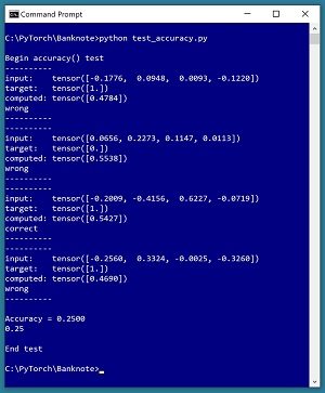
One of many possible implementations of an accuracy() function for the Banknote Authentication data and a short program to test the function is shown in Listing 4. The screenshot in Figure 2 shows the output from the test program. The first data item's target value is 1 and the computed output value is 0.4784 so the prediction is wrong (which isn't unexpected because the network has not been trained).
 [Click on image for larger view.] Figure 2: Output from the Test Program
Listing 4: A Model Accuracy Function
# test_accuracy.py

import numpy as np
import torch as T
device = T.device("cpu")

class BanknoteDataset(T.utils.data.Dataset): . . .
  # see Listing 1

class Net(T.nn.Module): . . .
  # see Listing 2

def accuracy(model, ds):
  # ds is a PyTorch Dataset
  # assumes model = model.eval()
  n_correct = 0; n_wrong = 0

  for i in range(len(ds)):
    inpts = ds[i]['predictors']
    target = ds[i]['target']
    with T.no_grad():
      oupt = model(inpts)

    print("----------")
    print("input:    " + str(inpts))
    print("target:   " + str(target))
    print("computed: " + str(oupt))

    # avoid 'target == 1.0'
    if target < 0.5 and oupt < 0.5:
      n_correct += 1
      print("correct")
    elif target >= 0.5 and oupt >= 0.5:
      n_correct += 1
      print("correct")
    else:
      n_wrong += 1
      print("wrong")

    print("----------")
  return (n_correct * 1.0) / (n_correct + n_wrong)

print("\nBegin accuracy() test ")

T.manual_seed(1)
np.random.seed(1)
train_file = ".\\Data\\banknote_k20_train.txt"
train_ds = BanknoteDataset(train_file, num_rows=4)

net = Net().to(device)
# net = net.train()
# train network

net = net.eval()
acc = accuracy(net, train_ds)
print("\nAccuracy = %0.4f" % acc)

print("\nEnd test ")
The accuracy() function is defined as an instance function so that it accepts a neural network model to evaluate and a PyTorch Dataset object that has been designed to work with the network. The idea here is that you created a Dataset object to use for training, and so you can use the Dataset to compute accuracy too.
The accuracy() function iterates through the Dataset object to process data items one at a time:
  for i in range(len(ds)):
    inpts = ds[i]['predictors']
    target = ds[i]['target']
    with T.no_grad():
      oupt = model(inpts)

. . .
Each item in a Dataset is a Dictionary object. Notice that the Dictionary keys of "predictors" and "target" are magic strings. Most PyTorch programs are tightly coupled like this. An alternative, more complex approach, is to parameterize the keys.
When iterating through a Dataset object in this way, the inpts tensor and the target tensor are both 1-dimensional vectors, which is fine even though during training the inputs, targets, and computed output objects are all 2-dimensional tensors. In other words, you can feed the Net object either a 2-dimensional tensor that holds multiple input items, or a 1-dimensional tensor that holds a single input item. Conceptually, this is similar to method overloading.
The output value is computed in a no_grad() block because there's no need for the computed oupt tensor to have a gradient since it isn't used for training. The predicted value is compared with the target value like so:
    if target < 0.5 and oupt < 0.5:
      n_correct += 1
      print("correct")
    elif target >= 0.5 and oupt >= 0.5:
      n_correct += 1
      print("correct")
    else:
      n_wrong += 1
      print("wrong")
The target value is 0.0 or 1.0 but I like to avoid comparing floating point values for exact equality so instead I check if the target value is less than 0.5 (which means it must be 0.0). Both target and oupt are PyTorch tensors that hold a single numeric value. In early versions of PyTorch, you had to use the item() method to extract the numeric values before comparing, like this:
if target.item() < 0.5 and oupt.item() < 0.5:
  . . .
But current versions of PyTorch allow you to directly compare tensors that have a single value.
The statements that call the accuracy function are:
net = Net().to(device)  # create network
net = net.eval()
acc = accuracy(net, train_ds)
print("\nAccuracy = %0.4f" % acc)
The neural network to evaluate is placed into eval() mode. If a neural network has a dropout layer or a batch normalization layer, you must set the network to train() mode during training and to eval() mode at all other times. In the case of the demo program, the neural network doesn't use dropout or batch normalization so you can omit setting the mode entirely. But in my opinion, it's good practice to explicitly set train() and eval() mode even when it's not technically necessary.
The accuracy() function iterates through a Dataset object one item at a time so that you can examine each item. A less flexible but more efficient design is to compute accuracy on the entire Dataset using a set operation approach:
def acc_coarse(model, ds):
  inpts = ds[:]['predictors']  # all rows
  targets = ds[:]['target']    # all target 0s and 1s
  with T.no_grad():
    oupts = model(inpts)       # all computed ouputs
  pred_y = oupts >= 0.5        # tensor of 0s and 1s
  num_correct = T.sum(targets==pred_y)  # tensor
  acc = (num_correct.item() * 1.0 / len(ds))  # scalar
  return acc
This approach is less clear but runs faster, so it's useful when you have a large Dataset and you only want the final accuracy result.
Saving a Trained Model
There are three main ways to save a PyTorch model to file: the older "full" technique, the newer "state_dict" technique, and the non-PyTorch ONNX technique. I recommend the "state_dict" technique which looks like:
  print("Saving trained model state dict ")
  path = ".\\Models\\banknote_sd_model.pth"
  T.save(net.state_dict(), path)
This code assumes that a subdirectory named Model exists relative to the program. The code should be mostly self-explanatory. It is common to use a ".pth" extenstion for a saved PyTorch model but you can use whatever you wish.
To load and use a saved model from a different file, you could write code like:
  model = Net().to(device)
  path = ".\\Models\\banknote_sd_model.pth"
  model.load_state_dict(T.load(path))
  x = T.tensor([[0.2, 0.,3, 0.6, 0.7]],
    dtype=T.float32)
  with T.no_grad():
    y = model(x)
  print("Prediction is " + str(y))
Notice that to load a saved PyTorch model from a program, the model's class definition must be defined in the program. In other words, when you save a trained model, you save the weights and biases but you don't save the model's definition. This seems a bit odd to most people who are new to PyTorch and are expecting a save() method to save everything instead of just the weights and biases.
There is an older "full" or "complete" technique to save a PyTorch model, but its name is rather misleading because it works just like the newer state_dict technique in the sense that code that uses the saved model must have access to the model's class definition. Using the older save technique looks very much like the state_dict technique but the older technique has some minor underlying technical problems which is why the newer technique was created. There is no reason to use the older technique except for backward compatibility.
A third way to save a trained PyTorch model is to use ONNX (Open Neural Network Exchange) technology. You can save a model with code like:
  path = ".\\Models\\banknote_onnx_model.onnx"
  dummy = T.tensor([[0.5, 0.5, 0.5, 0.5]],
    dtype=T.float32).to(device)
  T.onnx.export(net, dummy, path,
    input_names=["input1"],
    output_names=["output1"])
However, you cannot load a saved ONNX model using PyTorch. Instead, you must load the saved ONNX model and then use a special ONNX runtime in order to use the model. One example is:
  import onnx
  import onnxruntime
  import numpy as np

  path = ".\\Models\\banknote_onnx_model.onnx"
  model = onnx.load(path)
  onnx.checker.check_model(model)
  sess = onnxruntime.InferenceSession(path)

  x = np.array([[0.2, 0.3, 0.6, 0.7]],
    dtype=np.float32)
  y = sess.run(None, {"input1": x})
  print(y)  # prediction
ONNX is still relatively immature, so it's not fully supported by all neural network code libraries, and it has bugs when using complex neural models. ONNX is useful when you want a system to use a trained model but you don't want to expose the underlying neural network class definition.
Using a Trained Model
The last few statements in Listing 1 show an example of how to use a trained model. First, a NumPy matrix with just one input item is manually created:
  # 6. make a prediction
  raw_inpt = np.array([[4.4, 1.8, -5.6, 3.2]],
    dtype=np.float32)
  norm_inpt = raw_inpt / 20
  unknown = T.tensor(norm_inpt,
    dtype=T.float32).to(device)

  print("Setting normalized inputs to:")
  for x in norm_inpt[0]:
    print("%0.3f " % x, end="")
The demo code starts with NumPy data rather than a PyTorch tensor to illustrate the idea that in most cases input data is generated using Python rather than PyTorch. The input values are placed in a 2-dimensional matrix (indicated by the double square brackets) to illustrate the idea that you can feed a single input item or multiple input items to a trained model. The raw input values of (4.4, 1.8, -5.6, 3.2) are just dummy values that are similar to the pre-normalized source data. The input values are normalized by dividing by 20 because that's how the training and test data were normalized. After normalization, the input values are converted to a PyTorch tensor and then displayed to the shell.
Next, these statements make a prediction:
  net = net.eval()
  with T.no_grad():
    raw_out = net(unknown)    # a Tensor
  pred_prob = raw_out.item()  # scalar, [0.0, 1.0]
The net object is placed into eval() mode, which is good practice even when not necessary (when the model doesn't use dropout or batch normalization) because the default is train() mode. The input tensor is fed to the Net object in a no_grad() block because gradients are only needed during training. The result value is a PyTorch tensor with just a single value between 0.0 and 1.0. The numeric value in the tensor is extracted using the item() method to get an ordinary scalar value that is type Python float (64 bits).
The demo program concludes:
  print("\nPrediction prob = %0.6f " % pred_prob)
  if pred_prob < 0.5:
    print("Prediction = authentic")
  else:
    print("Prediction = forgery")
The demo program assumes that 0.5 is the boundary value that separates class 0 from class 1. This is standard practice but in some problem scenarios you might want to use a different boundary value such as 0.3 (which gives more class 1 predictions) or 0.8 (more class 0 predictions).
Wrapping Up
Learning how to create a PyTorch binary classifier usually can't be done in a strictly sequential manner. Based on my experience, most people need to use a spiral approach where they examine an overall program, then look at functional blocks of code such as defining the neural network and computing accuracy, and then examine the entire program again, and so on.
Creating and using neural networks using low-level code libraries such as PyTorch and TensorFlow gives you tremendous flexibility but is challenging. The difficulty of using TensorFlow led to the creation of the Keras library, which is essentially a high-level wrapper to make TensorFlow easier to use. I have seen several similar efforts to create a high-level wrapper library for PyTorch, but none of these wrapper libraries is being widely used at this time.
One of my job roles is to teach engineers and data scientists at my company how to use PyTorch. One of the most common questions from employee-students is how to use a trained PyTorch model from another system, such as a C# program or an ordinary Python program. The most common approach is to write custom code that uses the trained model weights and biases to compute output. The neural network input-output mechanism is relatively simple, and is all you need because no training needs to be performed.