The Data Science Lab
Neural Regression Using PyTorch: Model Accuracy
Dr. James McCaffrey of Microsoft Research explains how to evaluate, save and use a trained regression model, used to predict a single numeric value such as the annual revenue of a new restaurant based on variables such as menu prices, number of tables, location and so on.
The goal of a regression problem is to predict a single numeric value, for example, predicting the annual revenue of a new restaurant based on variables such as menu prices, number of tables, location and so on. There are several classical statistics techniques for regression problems. Neural regression solves a regression problem using a neural network. This article is the fourth in a series of four articles that present a complete end-to-end production-quality example of neural regression using PyTorch. The recurring example problem is to predict the price of a house based on its area in square feet, air conditioning (yes or no), style ("art_deco," "bungalow," "colonial") and local school ("johnson," "kennedy," "lincoln").
The process of creating a PyTorch neural network for regression consists of six steps:
- Prepare the training and test data
- Implement a Dataset object to serve up the data in batches
- Design and implement a neural network
- Write code to train the network
- Write code to evaluate the model (the trained network)
- Write code to save and use the model to make predictions for new, previously unseen data
Each of the six steps is complicated. And the six steps are tightly coupled which adds to the difficulty. This article covers the fifth and sixth steps -- evaluating, saving, and using a trained regression model.
A good way to see where this series of articles is headed is to take a look at the screenshot of the demo program in Figure 1. The demo begins by creating Dataset and DataLoader objects which have been designed to work with the house data. Next, the demo creates an 8-(10-10)-1 deep neural network. The demo prepares training by setting up a loss function (mean squared error), a training optimizer function (Adam) and parameters for training (learning rate and max epochs).
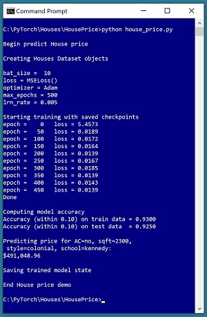 [Click on image for larger view.] Figure 1: Predicting the Price of a House Using Neural Regression
The demo trains the neural network for 500 epochs in batches of 10 items. An epoch is one complete pass through the training data. The training data has 200 items, therefore, one training epoch consists of processing 20 batches of 10 training items.
During training, the demo computes and displays a measure of the current error (also called loss) every 50 epochs. Because error slowly decreases, it appears that training is succeeding. Behind the scenes, the demo program saves checkpoint information after every 50 epochs so that if the training machine crashes, training can be resumed without having to start over from the beginning.
After training the network, the demo program computes the prediction accuracy of the model based on whether or not the predicted house price is within 10 percent of the true house price. The accuracy on the training data is 93.00 percent (186 out of 200 correct) and the accuracy on the test data is 92.50 percent (37 out of 40 correct). Because the two accuracy values are similar, it is likely that model overfitting has not occurred.
Next, the demo uses the trained model to make a prediction on a new, previously unseen house. The raw input is (air conditioning = "no", square feet area = 2300, style = "colonial", school = "kennedy"). The raw input is normalized and encoded as (air conditioning = -1, area = 0.2300, style = 0,0,1, school = 0,1,0). The computed output price is 0.49104896 which is equivalent to $491,048.96 because the raw house prices were all normalized by dividing by 1,000,000.
The demo program concludes by saving the trained model using the state dictionary approach. This is the most common of three standard techniques.
This article assumes you have an intermediate or better familiarity with a C-family programming language, preferably Python, but doesn't assume you know very much about PyTorch. The complete source code for the demo program, and the two data files used, are available in the download that accompanies this article. All normal error checking code has been omitted to keep the main ideas as clear as possible.
To run the demo program, you must have Python and PyTorch installed on your machine. The demo programs were developed on Windows 10 using the Anaconda 2020.02 64-bit distribution (which contains Python 3.7.6) and PyTorch version 1.7.0 for CPU installed via pip. You can find detailed step-by-step installation instructions for this configuration in my blog post.
The House Data
The raw House data is synthetic and was generated programmatically. There are a total of 240 data items, divided into a 200-item training dataset and a 40-item test dataset. The raw data looks like:
no    1275   bungalow   $318,000.00   lincoln
yes   1100   art_deco   $335,000.00   johnson
no    1375   colonial   $286,000.00   kennedy
yes   1975   bungalow   $512,000.00   lincoln
. . .
no    2725   art_deco   $626,000.00   kennedy
Each line of tab-delimited data represents one house. The value to predict, house price, is in 0-based column [3]. The predictors variables in columns [0], [1], [2] and [4] are air conditioning yes-no, area in square feet, architectural style and local school. For simplicity, there are just three house styles and three schools.
House area values were normalized by dividing by 10,000 and house prices were normalized by dividing by 1,000,000. Air conditioning was binary encoded as no = -1, yes = +1. Style was one-hot encoded as "art_deco" = (1,0,0), "bungalow" = (0,1,0), "colonial" = (0,0,1). School was one-hot encoded as "johnson" = (1,0,0), "kennedy" = (0,1,0), "lincoln" = (0,0,1). The resulting normalized and encoded data looks like:
-1   0.1275   0 1 0   0.3180   0 0 1
 1   0.1100   1 0 0   0.3350   1 0 0
-1   0.1375   0 0 1   0.2860   0 1 0
 1   0.1975   0 1 0   0.5120   0 0 1
. . .
-1   0.2725   1 0 0   0.6260   0 1 0
After the structure of the training and test files was established, I designed and coded a PyTorch Dataset class to read the house data into memory and serve the data up in batches using a PyTorch DataLoader object. A Dataset class definition for the normalized and encoded House data is shown in Listing 1.
Listing 1: A Dataset Class for the Student Data
class HouseDataset(T.utils.data.Dataset):
  # AC  sq ft   style  price   school
  # -1  0.2500  0 1 0  0.5650  0 1 0
  #  1  0.1275  1 0 0  0.3710  0 0 1
  # air condition: -1 = no, +1 = yes
  # style: art_deco, bungalow, colonial
  # school: johnson, kennedy, lincoln

  def __init__(self, src_file, m_rows=None):
    all_xy = np.loadtxt(src_file, max_rows=m_rows,
      usecols=[0,1,2,3,4,5,6,7,8], delimiter="\t",
      comments="#", skiprows=0, dtype=np.float32)

    tmp_x = all_xy[:,[0,1,2,3,4,6,7,8]]
    tmp_y = all_xy[:,5].reshape(-1,1)    # 2-D

    self.x_data = T.tensor(tmp_x, \
      dtype=T.float32).to(device)
    self.y_data = T.tensor(tmp_y, \
      dtype=T.float32).to(device)

  def __len__(self):
    return len(self.x_data)

  def __getitem__(self, idx):
    preds = self.x_data[idx,:]  # or just [idx]
    price = self.y_data[idx,:]
    return (preds, price)       # tuple of matrices
Preparing data and defining a PyTorch Dataset is not trivial. You can find the article that explains how to create Dataset objects and use them with DataLoader objects here.
The Neural Network Architecture
In the previous article in this series, I described how to design and implement a neural network for regression for the House data. One possible definition is presented in Listing 2. The code defines an 8-(10-10)-1 neural network with relu() activation on the hidden nodes.
Listing 2: A Neural Network for the Student Data
class Net(T.nn.Module):
  def __init__(self):
    super(Net, self).__init__()
    self.hid1 = T.nn.Linear(8, 10)  # 8-(10-10)-1
    self.hid2 = T.nn.Linear(10, 10)
    self.oupt = T.nn.Linear(10, 1)

    T.nn.init.xavier_uniform_(self.hid1.weight)
    T.nn.init.zeros_(self.hid1.bias)
    T.nn.init.xavier_uniform_(self.hid2.weight)
    T.nn.init.zeros_(self.hid2.bias)
    T.nn.init.xavier_uniform_(self.oupt.weight)
    T.nn.init.zeros_(self.oupt.bias)

  def forward(self, x):
    z = T.relu(self.hid1(x))
    z = T.relu(self.hid2(z))
    z = self.oupt(z)  # no activation
    return z
If you are new to PyTorch, the number of design decisions for a neural network can seem intimidating. But with every program you write, you learn which design decisions are important and which don't affect the final prediction model very much, and the pieces of the design puzzle eventually fall into place.
The Overall Program Structure
The overall structure of the PyTorch neural regression program, with a few minor edits to save space, is shown in Listing 3. I prefer to indent my Python programs using two spaces rather than the more common four spaces.
Listing 3: The Structure of the Demo Program
# house_price.py
# PyTorch 1.7.0-CPU Anaconda3-2020.02
# Python 3.7.6 Windows 10

import numpy as np
import time
import torch as T
device = T.device("cpu")

class HouseDataset(T.utils.data.Dataset):
  # AC  sq ft   style  price   school
  # -1  0.2500  0 1 0  0.5650  0 1 0
  #  1  0.1275  1 0 0  0.3710  0 0 1
  # air condition: -1 = no, +1 = yes
  # style: art_deco, bungalow, colonial
  # school: johnson, kennedy, lincoln

  def __init__(self, src_file, m_rows=None): . . .
  def __len__(self): . . .
  def __getitem__(self, idx): . . .

# ----------------------------------------------------

def accuracy(model, ds): . . .

# ----------------------------------------------------

class Net(T.nn.Module):
  def __init__(self): . . .
  def forward(self, x): . . .

# ----------------------------------------------------

def main():
  # 0. get started
  print("Begin predict House price ")
  T.manual_seed(4)
  np.random.seed(4)

  # 1. create Dataset and DataLoader objects
  # 2. create neural network
  # 3. train network
  # 4. evaluate model
  # 5. make a prediction
  # 6. save model
  print("End House price demo ")

if __name__== "__main__":
  main()
It's important to document the versions of Python and PyTorch being used because both systems are under continuous development. Dealing with versioning incompatibilities is a significant headache when working with PyTorch and is something you should not underestimate.
I like to use "T" as the top-level alias for the torch package. Most of my colleagues don't use a top-level alias and spell out "torch" many of times per program. Also, I use the full form of sub-packages rather than supplying aliases such as "import torch.nn.functional as functional." In my opinion, using the full form is easier to understand and less error-prone than using many aliases.
The demo program defines a program-scope CPU device object. I usually develop my PyTorch programs on a desktop CPU machine. After I get that version working, converting to a CUDA GPU system only requires changing the global device object to T.device("cuda") plus a minor amount of debugging.
The demo program defines just one helper method, accuracy(). All of the rest of the program control logic is contained in a single main() function. It is possible to define other helper functions such as train_net(), evaluate_model() and save_model(), but in my opinion this modularization approach unexpectedly makes the program more difficult to understand rather than easier to understand.
Saving Checkpoints
In almost all non-demo scenarios, it's a good idea to periodically save the state of the network during training so that if your training machine crashes, you can recover without having to start from scratch. The demo program shown running in Figure 1 saves checkpoints using these statements:
if epoch % 50 == 0:
  dt = time.strftime("%Y_%m_%d-%H_%M_%S")
  fn = ".\\Log\\" + str(dt) + str("-") + \
   str(epoch) + "_checkpoint.pt"
  info_dict = {
    'epoch' : epoch,
    'net_state' : net.state_dict(),
    'optimizer_state' : optimizer.state_dict()
  }
  T.save(info_dict, fn)
A checkpoint is saved every 50 epochs. A file name that looks like "2021_03_25-10_32_57-700_checkpoint.pt" is created. The file name contains the date (March 25, 2021), time (10:32 and 57 seconds AM), and epoch (700). The network state information is stored in a Dictionary object. The code assumes that there is an existing directory named Log. You must save the network state and the optimizer state. You can optionally save other information such as the epoch, and the states of the NumPy and PyTorch random number generators.
If the training machine crashes, you can recover training with code like:
fn = ".\\Log\\2021_03_25-10_32_57-700_checkpoint.pt"
chkpt = T.load(fn)
net = Net().to(device)
net.load_state_dict(chkpt['net_state'])
optimizer.load_state_dict(chkpt['optimizer_state'])
  . . .
epoch_saved = chkpt['epoch'] + 1
for epoch in range(epoch_saved, max_epochs):
  T.manual_seed(1 + epoch)
  # resume training as usual
If you want to recover training exactly as it would be if your machine hadn't crashed, which is usually the case, you must set the PyTorch random number generator seed value on each training epoch. This is necessary because DataLoader uses the PyTorch random number generator to serve up training items in a random order, and as of PyTorch version 1.7, there is no built-in way to save the state of a DataLoader object. If you don't set the PyTorch random seed in each epoch, you can recover from a crash. But the resulting training will be slightly different than if your machine had not crashed because the DataLoader will start using a different batch of training items.
Computing Model Accuracy
The most common approach for computing model accuracy for a regression problem is to calculate the number of predicted values that are within a specified percentage of the correct target values. For example, if a target price in the training data is 0.400 ($400,000) and the specified accuracy percentage is 10 percent, then a predicted price value between 0.360 and 0.440 would be logged as correct, but any other predicted price value would be logged as wrong.
In high level pseudo-code, computing accuracy looks like:
    loop thru each data item
      get item predictor input values
      get item target value
      use inputs to compute output value

      compute actual difference predicted, target
      compute max allowed difference
      if actual diff < max allowed
        correct prediction
      else
        wrong prediction
    end-loop
    return num correct / (num correct + num wrong)
One possible implementation of an accuracy() function for the House Price data, along with a short program to test the function, is shown in Listing 4. The screenshot in Figure 2 shows the output from the test program.
The first data item's predicted price is 0.0722 and the actual target price is 0.3000. The absolute value of the difference is 0.2278. The maximum allowed difference is 0.0300 and so the prediction is flagged as wrong. Of the six items, only the second and fifth items are predicted correctly. This isn't unexpected because the network has not been trained.
Listing 4: A Model Accuracy Function
# test_accuracy.py

import numpy as np
import torch as T
device = T.device("cpu")

# ----------------------------------------------------

class HouseDataset(T.utils.data.Dataset):
  # see Listing 1

class Net(T.nn.Module):
  # see Listing 2

# ----------------------------------------------------

def accuracy(model, ds, pct):
  n_correct = 0; n_wrong = 0

  for i in range(len(ds)):    # one item at a time
    (X, Y) = ds[i]            # (predictors, target)
    with T.no_grad():
      oupt = model(X)         # computed price

    print("-----------------------------")
    abs_delta = np.abs(oupt.item() - Y.item())
    max_allow = np.abs(pct * Y.item())
    print("predicted = %0.4f  actual = %0.4f \
 delta = %0.4f  max_allow = %0.4f : " % (oupt.item(),\
 Y.item(), abs_delta, max_allow),  end="")
    if abs_delta < max_allow:
      print("correct")
      n_correct +=1
    else:
      print("wrong")
      n_wrong += 1

  acc = (n_correct * 1.0) / (n_correct + n_wrong)
  return acc

# ----------------------------------------------------

print("Begin accuracy() test for House prices")

T.manual_seed(1)
np.random.seed(1)
train_file = ".\\Data\\houses_train.txt"
train_ds = HouseDataset(train_file, m_rows=6)

net = Net().to(device)
# net = net.train()
# train network

net = net.eval()
acc = accuracy(net, train_ds, 0.10)  # within 10%
print("\nAccuracy = %0.4f" % acc)
print("\nEnd test ")
The accuracy() function is defined as an instance function so that it accepts a neural network to evaluate and a PyTorch Dataset object that has been designed to work with the network. The idea here is that you created a Dataset object to use for training, and so you can use the Dataset to compute accuracy too.
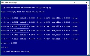 [Click on image for larger view.] Figure 2: Testing the Accuracy Function for House Price
The accuracy() function iterates through the Dataset object to process data items one at a time:
for i in range(len(ds)):    # one item at a time
  (X, Y) = ds[i]            # (predictors, target)
  with T.no_grad():
    oupt = model(X)         # computed price  . . .
Each item in a Dataset is a Tuple object, where the first part of the tuple holds the predictor values and the second holds the target price. When iterating through a Dataset object in this way, the X input tensor and the Y target tensor are both 1-dimensional vectors, which is fine even though during training the inputs, targets, and computed output objects are all 2-dimensional tensors. In other words, you can feed the Net object either a 2-dimensional tensor that holds multiple input items, or a 1-dimensional tensor that holds a single input item. Conceptually, this is similar to function overloading.
The output value is computed in a no_grad() block because there's no need for the computed output tensor to have a gradient since it isn't used for training.
The predicted house price is compared with the target price like so:
abs_delta = np.abs(oupt.item() - Y.item())
max_allow = np.abs(pct * Y.item())
if abs_delta < max_allow:
  n_correct +=1
else:
  n_wrong += 1
When a PyTorch tensor has just a single value, that value can be extracted using the item() method. In early versions of PyTorch, you had to use item() but current versions of PyTorch infer when you want to extract a single value. So, in the code above you could omit the call to the item() method. In my opinion, it's better to explicitly use the item() method in situations like this.
The statements that call the accuracy function are:
net = Net().to(device)
net = net.eval()
acc = accuracy(net, train_ds, 0.10)  # within 10% of true
print("\nAccuracy = %0.4f" % acc)
The neural network to evaluate is placed into eval() mode. If a neural network has a dropout layer or a batch normalization layer, you must set the network to train() mode during training and to eval() mode at all other times. In the case of the demo program, the neural network doesn't use dropout or batch normalization so you can omit setting the mode entirely. But in my opinion, it's good practice to explicitly set train() and eval() mode even when it's not technically necessary.
The eval() method operates by reference and so you can write just "net.eval()" rather than "net = net.eval()". I prefer using the net = net.eval() form, but I almost never see this form used.
The accuracy() function iterates through a Dataset object one item at a time so that you can examine each item. A less flexible but more efficient design is to compute accuracy on the entire Dataset using a set operation approach:
def accuracy_quick(model, dataset, pct):
  n = len(dataset)
  X = dataset[0:n][0]  # all predictor values
  Y = dataset[0:n][1]  # all target prices
  with T.no_grad():
    oupt = model(X)      # all computed prices
  max_deltas = T.abs(pct * Y)    # max allowable deltas
  abs_deltas = T.abs(oupt - Y)   # actual differences
  results = abs_deltas < max_deltas  # [[True, False, . .]]
  acc = T.sum(results, dim=0).item() / n  # dim not needed
  return acc
This approach is less clear but runs faster. The technique is useful when you have a large Dataset and you only want the final accuracy result, or when you are computing accuracy many times inside a loop.
Using a Trained Model
The demo program shown running in Figure 1 uses the trained model to make a prediction of new, previously unseen data. The input data is prepared like so:
net.eval()  # ugly but standard call form
print("Predicting price for AC=no, sqft=2300, ")
print(" style=colonial, school=kennedy: ")
unk = np.array([[-1, 0.2300,  0,0,1,  0,1,0]],
  dtype=np.float32)
unk = T.tensor(unk, dtype=T.float32).to(device)
The model is placed into eval() mode which is good practice even when not necessary (when the model doesn't use dropout or batch normalization) because the default is train() mode.
The demo input starts with NumPy data rather than a PyTorch tensor to illustrate the idea that in most cases input data is generated using Python rather than PyTorch. The input values are placed in a 2-dimensional matrix (indicated by the double square brackets) to illustrate the idea that you can feed a single input item or multiple input items to a trained model. The raw input values of ("no", 2300 square feet, "colonial", "kennedy") are normalized and encoded to (-1, 0.2300, 0,0,1, 0,1,0) in the same way that the training data was normalized and encoded.
Next, these statements make a prediction:
with T.no_grad():
  pred_price = net(unk)
pred_price = pred_price.item()  # scalar
str_price = \
  "${:,.2f}".format(pred_price * 1000000)
print(str_price)
The input tensor is fed to the Net object in a no_grad() block because gradients are only needed during training. The result value is a PyTorch tensor with a single value, which is extracted using the item() method. The predicted house price is displayed in un-normalized form by multiplying by 1,000,000.
Saving a Trained Model
There are three main ways to save a PyTorch model to file: the older "full" technique, the newer "state_dict" technique, and the non-PyTorch ONNX technique. I recommend the "state_dict" technique which looks like:
print("Saving trained model state dict ")
path = ".\\Models\\houses_model.pth"
T.save(net.state_dict(), path)
This code assumes that a subdirectory named Models exists relative to the program. The code should be mostly self-explanatory. It is common to use a ".pth" extension for a saved PyTorch model but you can use whatever you wish.
To load and use a saved model from a different program, you could write code like:
model = Net().to(device)
path = ".\\Models\\houses_model.pth"
model.load_state_dict(T.load(path))
x = T.tensor([[-1, 0.2300,  0,0,1,  0,1,0]],
  dtype=T.float32)
with T.no_grad():
  y = model(x)
print("Prediction is " + str(y))
Notice that to load a saved PyTorch model from a program, the model's class definition must be defined in the program. In other words, when you save a trained model, you save the weights and biases but you don't save the model's definition. This seems a bit odd to most people who are new to PyTorch and are expecting a save() method to save everything instead of just the weights and biases.
There is an older "full" or "complete" technique to save a PyTorch model, but its name is rather misleading because it works just like the newer state_dict technique in the sense that code that uses the saved model must have access to the model's class definition. Using the older save technique looks very much like the state_dict technique but the older technique has some minor underlying technical problems which is why the newer technique was created. There is no reason to use the older technique except for backward compatibility.
A third way to save a trained PyTorch model is to use ONNX (Open Neural Network Exchange) technology. You can save a model with code like:
path = ".\\Models\\houses_onnx_model.onnx"
dummy = T.tensor([[1, 0.5, 1,0,0, 0,1,0]],
  dtype=T.float32).to(device)
T.onnx.export(net, dummy, path,
  input_names=["input1"],
  output_names=["output1"])
However, you cannot load a saved ONNX model using PyTorch program. Instead, you must load the saved ONNX model and then use a special ONNX runtime. One example is:
import onnx
import onnxruntime
import numpy as np

path = ".\\Models\\student_onnx_model.onnx"
model = onnx.load(path)
onnx.checker.check_model(model)
sess = onnxruntime.InferenceSession(path)

x = T.tensor([[-1, 0.2300,  0,0,1,  0,1,0]],
  dtype=T.float32)
y = sess.run(None, {"input1": x})
print(y)  # prediction
ONNX is still relatively immature so it's not fully supported by all neural network code libraries, and it has some bugs when using complex neural models. ONNX is useful when you want a system to use a trained model but you don't want to expose the underlying neural network class definition.
Wrapping Up
Learning how to create a PyTorch neural regression system usually can't be done in a strictly sequential manner. Based on my experience, most people need to use a spiral approach where they examine an overall program, then look at functional blocks of code such as defining the neural network and computing accuracy, and then examine the entire program again, and so on.
Creating and using neural networks using low-level code libraries such as PyTorch and TensorFlow gives you tremendous flexibility but is challenging. The difficulty of using TensorFlow led to the creation of the Keras library, which is essentially a high-level wrapper to make TensorFlow easier to use. I have seen several similar efforts to create a high-level wrapper library for PyTorch, but none of these wrapper libraries is being widely used at this time.