The Data Science Lab

Generating Synthetic Data Using a Variational Autoencoder with PyTorch

Generating synthetic data is useful when you have imbalanced training data for a particular class, for example, generating synthetic females in a dataset of employees that has many males but few females.

• By James McCaffrey
• 05/07/2021

A variational autoencoder (VAE) is a deep neural system that can be used to generate synthetic data. VAEs share some architectural similarities with regular neural autoencoders (AEs) but an AE is not well-suited for generating data. Generating synthetic data is useful when you have imbalanced training data for a particular class. For example, in a dataset of tech company employee information, you might have many male developer employees but very few female employees. You could train a VAE on the female employees and use the VAE to generate synthetic women.

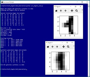
A good way to see where this article is headed is to take a look at the screenshot of a demo program in Figure 1. The demo generates synthetic images of handwritten "1" digits based on the UCI Digits dataset. Each image is 8 by 8 pixel values between 0 and 16. The demo uses image data but VAEs can generate synthetic data of any kind. The demo begins by loading 389 actual "1" digit images into memory. A typical "1" digit from the training data is displayed. Next, the demo trains a VAE model using the 389 images. The demo concludes by using the trained VAE to generate a synthetic "1" image and displays its 64 numeric values and its visual representation.

This article assumes you have an intermediate or better familiarity with a C-family programming language, preferably Python, and a basic familiarity with the PyTorch code library. The source code for the demo program is a bit too long to present in its entirety in this article, but the complete code and training data are available in the accompanying file download. (The training data is embedded in commented-form in the source code).

VAEs are fairly complex, both conceptually and technically, so this article focuses on explaining the key ideas you need to understand in order to create VAEs to suit your problem scenarios. All normal error checking code has been omitted to keep the main ideas as clear as possible.

To run the demo program, you must have Python and PyTorch installed on your machine. The demo programs were developed on Windows 10 using the Anaconda 2020.02 64-bit distribution (which contains Python 3.7.6) and PyTorch version 1.8.0 for CPU installed via pip. Installation is not trivial. You can find detailed step-by-step installation instructions for this configuration in my blog post.

The UCI Digits Dataset
The UCI Digits dataset is a 3,823-item file named optdigits.tra (intended for training) and a 1,797-item file named optdigits.tes (for testing). I downloaded the files and renamed them to optdigits_train_3823.txt and optdigits_test_1797.txt. Each file is a simple, comma-delimited text file. Each line represents an 8 by 8 handwritten digit from "0" to "9."

The UCI Digits data looks like:

0,1,6,16,12, . . . 1,0,0,13,0
2,7,8,11,15, . . . 16,0,7,4,1
. . .

The first 64 values on each line are the image pixel values. Each pixel is a grayscale value between 0 and 16. The last value on each line is the digit/label. There are about 380 of each digit in the training file and about 180 of each digit in the test file, but the digits are not evenly distributed. The counts of each "0" through "9" digit in the training data are: 376, 389, 380, 389, 387, 376, 377, 387, 380 and 382.

I wrote a short utility program to scan through the training data file and filter out the 389 "1" digits and save them as file uci_digits_1_only.txt using the same comma-delimited format.

The demo program defines a PyTorch Dataset class to load the data in memory. See Listing 1.

Listing 1: A Dataset Class for the UCI Digits Data

import torch as T
import numpy as np

class UCI_Digits_Dataset(T.utils.data.Dataset):
  # like: 8,12,0,16, . . 15,7
  # 64 pixel values [0-16], digit [0-9]

  def __init__(self, src_file, n_rows=None):
    tmp_x = np.loadtxt(src_file, max_rows=n_rows,
      usecols=range(0,64), delimiter=",", comments="#",
      dtype=np.float32)  # just pixels, no labels
    tmp_x /= 16.0        # normalize
    self.x_data = T.tensor(tmp_x, 
      dtype=T.float32).to(device) 

  def __len__(self):
    return len(self.x_data)

  def __getitem__(self, idx):
    return self.x_data[idx]

The class loads a file of UCI digits data into memory as a two-dimensional array using the NumPy loadtxt() function. The pixel values are normalized to a range of 0.0 to 1.0 by dividing by 16, which is important for VAE architecture. The NumPy array is converted to a PyTorch tensor

The Dataset can be used with code like this:

fn = ".\\Data\\ uci_digits_1_only.txt "
my_ds = UCI_Digits_Dataset(fn)
my_ldr = T.utils.data.DataLoader(my_ds, \
  batch_size=10, shuffle=True)
for (b_ix, batch) in enumerate(my_ldr):
  # b_ix is the batch index
  # batch has 10 items with 64 values between 0 and 1
. . .

The Dataset object is passed to a built-in PyTorch DataLoader object. The DataLoader object serves up the data in batches of a specified size, in a random order on each pass through the Dataset.

The design pattern presented here will work for most variational autoencoder data generation scenarios. If your raw data contains a categorical variable, such as "color" with possible values "red," "blue" or "green," you can one-hot encode the data: "red" = (1.0, 0.0, 0.0), "blue" = (0.0, 1.0, 0.0), "green" = (0.0, 0.0, 1.0).

Understanding Variational Autoencoders
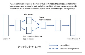
Variational autoencoders are complex. My explanation will take some liberties with terminology and details to help make the explanation digestible. The diagram in Figure 2 shows the architecture of the 64-32-[4,4]-4-32-64 VAE used in the demo program. An input image x, with 64 values between 0 and 1, is fed to the VAE. A neural layer condenses the 64-values down to 32 values. The 32 values are condensed to two tensors, each with four values. The first tensor represents the mean of the distribution of the source data. The second tensor represents the standard deviation of the distribution. For technical reasons the standard deviation is stored as the log of the variance. You might recall from statistics that standard deviation is the square root of variance. Using the log of the variance helps prevent values from becoming excessively large.

The key point is that a VAE learns the distribution of its source data rather than memorizing the source data. A data distribution is just description of the data, given by its mean (average value) and standard deviation (measure of spread).

The mean and standard deviation (in the form of log-variance) are combined statistically to give a tensor with four values called the latent representation. These four values represent the core information contained in a digit image. The four values of the latent representation are expanded to 32 values, and those 32 values are expanded to 64 values called the reconstruction of the input.

Defining a Variational Autoencoder
The demo code that defines a VAE that corresponds Figure 2 is presented in Listing 2. The __init__() method defines the five neural network layers used by the system. For simplicity, the demo uses default initialization of weights and biases.

The encode() method accepts an input image, in the form of a tensor with 64 values. Those values are condensed to 32 values and then condensed to a pair of tensors with four values. Designing the architecture for a VAE requires trial and error guided by experience.

Listing 2: Variational Autoencoder Definition

class VAE(T.nn.Module):
  def __init__(self):
    super(VAE, self).__init__()
    # 64-32-[4,4]-4-32-64

    self.input_dim = 64
    self.latent_dim = 4

    self.fc1 = T.nn.Linear(64, 32)
    self.fc2a = T.nn.Linear(32, 4)  # mean
    self.fc2b = T.nn.Linear(32, 4)  # log-var
    self.fc3 = T.nn.Linear(4, 32)
    self.fc4 = T.nn.Linear(32, 64)

    # TODO: explicit weight initialization

  # encode: 64-32-[4,4]
  def encode(self, x):
    z = T.sigmoid(self.fc1(x))       # 64-32
    mean = T.sigmoid(self.fc2a(z))   # 32-4
    logvar = T.sigmoid(self.fc2b(z)) # 32-4           
    return (mean, logvar)

  # decode: 4-32-64
  def decode(self, z): 
    z = T.sigmoid(self.fc3(z))   # 4-32
    z = T.sigmoid(self.fc4(z))   # 32-64
    return z

  # forward: encode + combine + decode
  # 64-32-[4,4]-4-32-64
  def forward(self, x):
    (mean, logvar) = self.encode(x)   # 4-4
    stdev = T.exp(0.5 * logvar)
    noise = T.randn_like(stdev)
    inpt = mean + (noise * stdev)     # 4
    recon_x = self.decode(inpt)       # 4-32-64
    return (recon_x, mean, logvar)

The decode() method assumes that the mean and log-variance, each with four values, have been combined in some way to give a latent representation with four values. Those four values are expanded to 32 values and then to 64 values.

The forward() method first calls encode(), which yields a mean and log-variance. They are combined by these three statements:

stdev = T.exp(0.5 * logvar)
noise = T.randn_like(stdev)
inpt = mean + (noise * stdev)

First, the log-variance is converted to standard deviation. The math is a bit tricky. Next, four random values that are Gaussian distributed with mean = 0.0 and standard deviation = 1.0 are generated by the randn_like() function. The randn part of the function name stands for "random, normal." The _like part of the name means "with the same shape and data type."

Combining the mean and log-variance in this way is called the reparameterization trick. The discovery of this idea in the original 2013 research paper ("Auto-Encoding Variational Bayes" by D.P. Kingma and M. Welling) was the key to enabling VAEs in practice.

Training a Variational Autoencoder
Training a VAE involves two measures of similarity (or equivalently measures of loss). First, you must measure how closely the reconstructed output matches the source input. More concretely, the 64 output values should be very close to the 64 input values. Because the input values are normalized to between 0.0 and 1.0, the design of the VAE should ensure that the output values are also between 0.0 and 1.0 by using sigmoid() or relu() activation. Because both input and output values are between 0.0 and 1.0, the training code can use either binary cross entropy or mean squared error to compare input and output values.

The second part of training a VAE measures how likely it is that the output values could be produced by the distribution defined by the mean and log-variance. For example, a distribution of people's heights might have a mean of 70.0 inches and a standard deviation of 4.0 inches. A person who is 71.0 inches tall would not be unexpected. But a person who is 80.0 inches tall is not likely to have come from the distribution.

There are many techniques from classical statistics that can be used to measure how likely it is that a data item comes from a particular distribution. The technique used most often when training a VAE is called Kullback-Leibler (KL) divergence. Small KL divergence values indicate that a data item is likely to have come from a distribution, and large KL divergence values indicate unlikely.

The demo program defines the loss function for training a VAE as:

def cus_loss_func(recon_x, x, mean, logvar, beta=1.0):
  # aka ELBO (evidence lower bound loss)
  # see: https://arxiv.org/abs/1312.6114
  bce = T.nn.functional.binary_cross_entropy(recon_x, x, \
    reduction="sum")
  kld = -0.5 * T.sum(1 + logvar - T.pow(mean, 2) - \
    T.exp(logvar))
  return bce + (beta * kld)  # beta weights KLD component

The loss function first computes binary cross entropy loss between the source x and the reconstructed x and stores that single tensor value as bce. Next the KL divergence is computed using a clever statistics shortcut that assumes the distribution is Gaussian (i.e., normal or bell-shaped). This assumption is not always true, but the technique works well in practice.

The binary cross entropy measure of error value is combined with the KL divergence measure of error value by adding, with a constant called beta to control the weight given to the KL divergence component. A beta value of 1.0 is the default and weights the binary cross entropy and KL divergence values equally.

With the loss function defined, the demo program defines a train() function for the VAE using the code in Listing 3. Training a VAE is similar in most respects to training a regular neural system. The main difference is that the output from calling the VAE consists of a tuple of three values: the internal mean and log-variance, which are needed by the KL divergence part of the custom loss function and the reconstructed x, which is needed by both the KL divergence and binary cross entropy part of the loss function.

Listing 3: Training a Variational Autoencoder

def train(vae, ds, bs, me, le, lr, beta):
  # model, dataset, batch_size, max_epochs,
  # log_every, learn_rate, loss KLD weighting
  vae.train()  # set mode
  data_ldr = T.utils.data.DataLoader(ds, batch_size=bs,
    shuffle=True)
  opt = T.optim.Adam(vae.parameters(), lr=lr)
  print("\nStarting training")
  for epoch in range(0, me):
    epoch_loss = 0.0
    for (bat_idx, batch) in enumerate(data_ldr):
      opt.zero_grad()
      (recon_x, mean, logvar) = vae(batch)
      loss_val = cus_loss_func(recon_x, batch, mean, \
        logvar, beta)
      loss_val.backward()
      epoch_loss += loss_val.item()  # average per batch
      opt.step()
    if epoch % le == 0:
      print("epoch = %4d   loss = %0.4f" % (epoch, epoch_loss))
  print("Done ")

The train() function is prepared by setting up its argument values and is called like so:

vae = VAE().to(device)  # create model
bat_size = 10
max_epochs = 10
log_interval = 2
lrn_rate = 0.001
beta = 1.0  # weight of KLD component of loss

train(vae, data_ds, bat_size, max_epochs, 
  log_interval, lrn_rate, beta)

The train() function uses the Adam optimization method. In general Adam usually works well, but in some of my experiments, basic stochastic gradient descent with a decaying learning rate schedule works better.

Using the VAE to Generate Synthetic Data
After the VAE has been trained, the demo program uses it to generate a synthetic "1" digit image using these statements:

vae.eval()
for i in range(1):
  rinpt = T.randn(1, vae.latent_dim).to(device)
  with T.no_grad():
    si = vae.decode(rinpt).numpy()
  si = np.rint(si * 16)

  print("\nSynthetic generated image (de-normed): ")
  print(si) 
  display_digit(si)

The VAE model is set into evaluation mode. Technically this is not necessary because the VAE doesn't use dropout or batch normalization, but explicitly setting the mode is good practice in my opinion.

In most situations you'll want to generate many synthetic data items. The demo generates just one synthetic image to keep the size of the screenshot in Figure 1 small. A random tensor with four Gaussian (normal) values is created using the randn() function. The decode() method accepts the four random values, and expands them to 64 pixel values between 0.0 and 1.0 which are then converted to a NumPy array. Recall that a source UCI Digits image has 64 values between 0 and 16, but the values are normalized by the Dataset object. The 64 output values between 0.0 and 1.0 are de-normalized by multiplying them by 16 and applying the rint() function ("round to integer").

The resulting synthetic digit image is displayed by a program-defined display_digit() function:

import matplotlib.pyplot as plt
def display_digit(x, save=False):
  pixels = x.reshape((8,8))  
  plt.imshow(pixels, cmap=plt.get_cmap('gray_r'))
  if save == True:
    plt.savefig(".\\idx_" + str(idx) + "_digit_" + \
    str(label) + ".jpg", bbox_inches='tight')
  plt.show() 
  plt.close()

Because the demo data represents images, you can get an intuitive idea of how well the VAE works by checking the synthetic data by eye. For non-image source data, you'd need to examine the synthetic data in whatever way makes sense for your problem scenario.

Wrapping Up
Even though variational autoencoders have been studied for several years, there are many ideas that are not well understood. For example, in the early days of neural networks, it was not known if an exotic hidden layer activation function such as arctan() would have a big effect (it doesn't). Similarly, it's not known, at least to the best of my knowledge, what effect alternatives to KL divergence, and alternatives to the assumption of a Gaussian distribution, might have.

There are several other ways to generate synthetic data. A crude technique is to take an existing data item and then permute it slightly by adding small random values. However, this approach is not vey principled and there's no way of knowing if a slight change in a predictor value could have a big change in the item's class label.

A synthetic data generation technique which is somewhat related to VAE generation is to use a generative adversarial network (GAN). GANs were introduced in 2014, and like VAEs, have many ideas that are not well understood. Based on my experience, VAEs are somewhat easier to work with than GANs.

• Get Code Download