The Data Science Lab
Spiral Dynamics Optimization with Python
Dr. James McCaffrey of Microsoft Research explains how to implement a geometry-inspired optimization technique called spiral dynamics optimization (SDO), an alternative to Calculus-based techniques that may reach their limits with huge neural networks.
Training a neural network is the process of finding good values for the network's weights and biases. Put another way, training a neural network is the process of using an optimization algorithm of some sort to find values for the weights and biases that minimize the error between the network's computed output values and the known correct output values from the training data.
By far the most common form of optimization for neural network training is stochastic gradient descent (SGD). SGD has many variations including Adam (adaptive momentum estimation), Adagrad (adaptive gradient), and so on. All SGD-based optimization algorithms use the Calculus derivative (gradient) of an error function. But there are dozens of alternative optimization techniques that don't use gradients. Examples include bio-inspired optimization techniques such as genetic algorithms and particle swarm optimization, and geometry-inspired techniques such as Nelder-Mead (also known as simplex, or amoeba method).
This article explains how to implement a geometry-inspired optimization technique called spiral dynamics optimization (SDO). A good way to see where this article is headed is to take a look at the screenshot of a demo program in Figure 1. The demo program uses SDO to solve the Rosenbrock function in three dimensions.
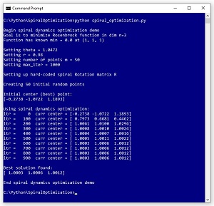 [Click on image for larger view.] Figure 1: Using Spiral Dynamics Optimization to Solve the Rosenbrock Function.
The Rosenbrock function with dim = 3 has a known solution of 0.0 at (1, 1, 1). The demo program sets up m = 50 random points where each point is a possible solution. SDO has two parameters: theta set to pi / 3 = 1.0472 and r set to 0.98. These parameters will be explained shortly. The demo program iterates 1,000 times. On each iteration, each of the 50 possible solution points moves towards the current best-known solution according to spiral geometry. After 1,000 iterations, the best solution found is at (1.0003, 1.0006, 1.0012) which is quite close to the true solution at (1, 1, 1).
This article assumes you have an intermediate or better familiarity with a C-family programming language. The demo program is implemented using Python but you should have no trouble refactoring to another language such as C# or JavaScript if you wish.
The complete source code for the demo program is presented in this article and is also available in the accompanying file download. All normal error checking has been removed to keep the main ideas as clear as possible.
To run the demo program, you must have Python installed on your machine. The demo program was developed on Windows 10 using the Anaconda 2020.02 64-bit distribution (which contains Python 3.7.6). The demo program has no significant dependencies so any relatively recent version of Python 3 will work fine.
The Rosenbrock Function
The Rosenbrock function is a standard benchmark problem for optimization algorithms. The Rosenbrock function can be defined for dimension = 2 or higher. The equation is f(x) = Sum [ 100 * (x(i+1) - x(i)^2 + (1 - x(i))^2 ]. The graph in Figure 2 shows the Rosenbrock function for dim = 2 where the minimum value is 0.0 at (1, 1). The Rosenbrock function is challenging because it's easy to get close to the minimum but then the surface becomes very flat and it's difficult to make progress.
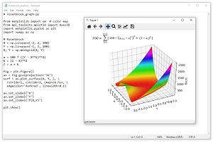 [Click on image for larger view.] Figure 2: The Rosenbrock Function for dim = 2.
Understanding Spiral Dynamics
The basic ideas of spiral dynamics for dim = 2 are shown in an example in Figure 3. There is a fixed center located at (0, 0). A single point starts at k = 0 at position (10, 10). The point moves in a counterclockwise direction through an angle theta = pi / 4 and then shrinks towards the center by a distance factor of 0.90 to reach k = 1 at (0.00, 12.73).
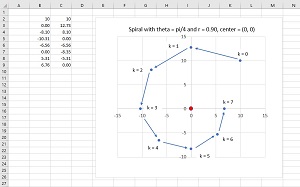 [Click on image for larger view.] Figure 3: Spiral Dynamics for dim = 2.
The process continues. On each iteration, the point moves by an angle theta and then towards the center. The net effect is that the point spirals in towards the center. The angle theta controls how curved the spiral is. Small values of theta give a very smooth curve. Large values of theta give a more boxy, rectangular shape. The shrink factor r controls how quickly the spiral moves towards the center. Large values of r, close to 1, don't move a point towards the center as quickly as smaller values of r such as 0.80.
Given an angle theta and a shrink factor r, it is possible to compute a new location of a point at (x, y) by multiplying the point by the rotation matrix R given by:
r * R = [ cos(theta)  -sin(theta) ]
        [ sin(theta)   cos(theta) ]
This is not at all obvious and can be considered a magic equation for spiral dynamics optimization. This rotation matrix is called R12 in research literature, which means it spirals a point in dimensions 1 and 2.
To spiral in dim = 2 is very easy. To spiral in higher dimensions you must compose multiple R matrices. For dim = 3 you compute like so (omitting the theta):
R12 = [cos  -sin     0]
      [sin   cos     0]
      [0     0       1]

R13 = [cos   0    -sin]
      [0     1       0]
      [sin   0     cos]

R23 = [1     0       0]
      [0     cos  -sin]
      [0     sin   cos]

R = R23 * R13 * R12 (compose)
R = r * R  (scale)
If you examine the example carefully, you'll see the pattern.
Instead of just one point moving in a spiral motion towards a fixed center, spiral dynamics optimization uses multiple points. On each iteration the best point is identified and used as the center that all points spiral towards. On the next iteration, a new center is found, and the process continues.
The Demo Program
The complete source code for the demo program is presented in Listing 1. The program defines three helper functions: rosenbrock_error(), find_center(), and move_point(). All the control logic is in a single main() function. Two additional helper functions -- make_Rab() and make_R() -- are not used by the demo but are needed for non-demo scenarios.
Listing 1: Complete Spiral Dynamics Optimization Demo Code
# spiral_optimization.py
# Anaconda3-2020.02  Python 3.7.6  NumPy 1.19.5
# Windows 10
# minimize Rosenbrock dim=3 using spiral optimization

import numpy as np

def rosenbrock_error(x, dim):
  # min val = 0.0 at [1,1,1, . . 1]
  dim = len(x)
  z = 0.0
  for i in range(dim-1):
    a = 100 * ((x[i+1] - x[i]**2)**2)
    b = (1 - x[i])**2
    z += a + b
  err = (z - 0.0)**2
  return err

def find_center(points, m):
  # center is point with smallest error
  # note: m = len(points) (number of points)
  n = len(points[0])  # n = dim
  best_err = rosenbrock_error(points[0], n)
  idx = 0
  for i in range(m):
    err = rosenbrock_error(points[i], n)
    if err < best_err:
      idx = i; best_err = err
  return np.copy(points[idx])

def move_point(x, R, RminusI, center):
  # move x vector to new position, spiraling around center
  # note: matmul() automatically promotes vector to matrix
  offset = np.matmul(RminusI, center)
  new_x = np.matmul(R, x) - offset
  return new_x

def make_Rab(a, b, n, theta):
  # make Rotation matrix, dim = n, a, b are 1-based
  # helper for make_R() function
  a -= 1; b -= 1  # convert a,b to 0-based
  result = np.zeros((n,n))
  for r in range(n):
    for c in range(n):
      if r == a and c == a: result[r][c] = np.cos(theta)
      elif r == a and c == b: result[r][c] = -np.sin(theta)
      elif r == b and c == a: result[r][c] = np.sin(theta)
      elif r == b and c == b: result[r][c] = np.cos(theta)
      elif r == c: result[r][c] = 1.0
  return result

def make_R(n, theta):
  result = np.zeros((n,n))
  for i in range(n):
    for j in range(n):
      if i == j: result[i][j] = 1.0  # Identity
  for i in range(1,n):
    for j in range(1,i+1):
      R = make_Rab(n-i, n+1-j, n, theta)
      result = np.matmul(result, R)  # compose
  return result

def main():
  print("\nBegin spiral dynamics optimization demo ")
  print("Goal is to minimize Rosenbrock function in dim n=3")
  print("Function has known min = 0.0 at (1, 1, 1) ")

  # 0. prepare
  np.set_printoptions(precision=4, suppress=True, sign=" ")
  np.set_printoptions(formatter={'float': '{: 0.4f}'.format})
  np.random.seed(4)

  theta = np.pi/3  # radians. small = curved, large = squared
  r = 0.98  # closer to 1 = tight spiral, closer 0 = loose
  m = 50    # number of points / possible solutions
  n = 3     # problem dimension
  max_iter = 1000

  print("\nSetting theta = %0.4f " % theta)
  print("Setting r = %0.2f " % r)
  print("Setting number of points m = %d " % m)
  print("Setting max_iter = %d " % max_iter)

  # 1. set up the Rotation matrix for n=3
  print("\nSetting up hard-coded Rotation matrix R ")

  ct = np.cos(theta)
  st = np.sin(theta)
  R12 = np.array([[ct,  -st,    0],
                  [st,   ct,    0],
                  [0,     0,    1]])

  R13 = np.array([[ct,   0,   -st],
                  [0,    1,     0],
                  [st,   0,    ct]])

  R23 = np.array([[1,    0,     0],
                  [0,    ct,  -st],
                  [0,    st,   ct]])

  R = np.matmul(R23, np.matmul(R13, R12))  # compose
  # R = make_R(3, theta)  # programmatic approach

  R = r * R  # scale / shrink

  I3 = np.array([[1,0,0], [0,1,0], [0,0,1]])
  RminusI = R - I3

  # 2. create m initial points and find best point
  print("\nCreating %d initial random points " % m)
  points = np.random.uniform(low=-5.0, \
    high=5.0, size=(m, 3))

  center = find_center(points, m)
  print("\nInitial center (best) point: ")
  print(center)

  # 3. spiral points towards center, update center
  print("\nUsing spiral dynamics optimization: ")
  for itr in range(max_iter):
    if itr % 100 == 0:
      print("itr = %5d  curr center = " % itr, end="")
      print(center)
    for i in range(m):  # move each point toward center
      x = points[i]
      points[i] = move_point(x, R, RminusI, center)
      # print(points); input()
    center = find_center(points, m)  # find new center

  # 4. show best center found
  print("\nBest solution found: ")
  print(center)

  print("\nEnd spiral dynamics optimization demo ")

if __name__ == "__main__":
  main()
The demo defines a rosenbrock_error() function that accepts a vector of values, x, then computes the Rosenbrock function for x, and then returns the squared difference between the computed value and the known correct value of 0.0:
def rosenbrock_error(x, dim):
  # min val = 0.0 at [1,1,1, . . 1]
  dim = len(x)
  z = 0.0
  for i in range(dim-1):
    a = 100 * ((x[i+1] - x[i]**2)**2)
    b = (1 - x[i])**2
    z += a + b
  err = (z - 0.0)**2
  return err
Notice that because the true minimum value of the Rosenbrock function is 0.0, it's not really necessary to subtract it from the computed value before squaring.
After each iteration, when all points have been moved in a spiral motion, the new best solution / point is found by function find_center() defined as:
def find_center(points, m):
  n = len(points[0])  # n = dim
  best_err = rosenbrock_error(points[0], n)
  idx = 0
  for i in range(m):
    err = rosenbrock_error(points[i], n)
    if err < best_err:
      idx = i; best_err = err
  return np.copy(points[idx])
The function accepts an array-of-arrays parameter, named points, that holds all current possible solutions. The m parameter is the number of points. That value could be computed as len(points) but in optimization research it's common to pass m explicitly anyway.
The Main Function
The main() function begins by setting up the program parameters. SDO is very sensitive to the values used for m (number of points / solutions), theta (spiral angle), and r (spiral shrink factor). Parameter sensitivity means that you must do a significant amount of experimentation to get good results. Parameter sensitivity is a weakness of SDO but is also a weakness of gradient-based optimization techniques such as SGD.
def main():
  # 0. prepare
  np.set_printoptions(precision=4, suppress=True, sign=" ")
  np.set_printoptions(formatter={'float': '{: 0.4f}'.format})
  np.random.seed(4)

  theta = np.pi/3  # radians. small = curved, large = squared
  r = 0.98  # closer to 1 = tight spiral, closer 0 = loose
  m = 50    # number of points / possible solutions
  n = 3     # problem dimension
  max_iter = 1000
. . .
After setting up parameters, the demo program hard-codes the first of the three R matrices needed for a dim = 3 problem:
  # 1. set up the Rotation matrix for n=3
  print("\Setting up spiral Rotation matrix R ")

  ct = np.cos(theta)
  st = np.sin(theta)
  R12 = np.array([[ct,  -st,    0],
                  [st,   ct,    0],
                  [0,     0,    1]])
This approach is fine for dim = 3, but for a problem with a larger dim, such as dim = 5, you'd have to hard-code Choose(5,2) = 10 matrices: R12, R13, R14, R15, R23, R24, R25, R34, R35, R45. A programmatic approach will be presented shortly.
Next, the R13 and R23 matrices are manually constructed, composed together, and shrunk:
  R13 = np.array([[ct,   0,   -st],
                  [0,    1,     0],
                  [st,   0,    ct]])

  R23 = np.array([[1,    0,     0],
                  [0,    ct,  -st],
                  [0,    st,   ct]])

  R = np.matmul(R23, np.matmul(R13, R12))  # compose
  R = r * R  # scale / shrink
Again, a hard-coded approach like this is only feasible for dim = 3 or maybe dim = 4 if you don't mind a lot of typing.
It turns out that spiraling in n dimensions requires R minus the Identity matrix. The Identity matrix for dim = 3 is a matrix with 1s on the main diagonal, 0s elsewhere:
  I3 = np.array([[1,0,0], [0,1,0], [0,0,1]])
  RminusI = R - I3
Next, the demo initializes a set of m random points and finds the best of these initial points:
  # 2. create m initial points and
  # find curr center (best point)
  print("\nCreating %d initial random points " % m)
  points = np.random.uniform(low=-5.0, high=5.0,
    size=(m, 3))

  center = find_center(points, m)
  print("\nInitial center (best) point: ")
  print(center)
The main processing loop is surprisingly short:
  print("\nUsing spiral dynamics optimization: ")
  for itr in range(max_iter):
    if itr % 100 == 0:
      print("itr = %5d  curr center = " % itr, end="")
      print(center)
    for i in range(m):  # move each pt toward center
      x = points[i]
      points[i] = move_point(x, R, RminusI, center)
      # print(points); input()
    center = find_center(points, m)  # find new center
The move_point() function moves each point towards the current best center. The RminusI matrix does not change and so it's passed in as an argument so that it doesn't have to be re-computed on each iteration.
The demo concludes by displaying the best solution found:
. . .
  # 4. show best center found
  print("\nBest solution found: ")
  print(center)
  print("\nEnd spiral dynamics optimization demo ")
if __name__ == "__main__":
  main()
There are several ways you can enhance the output. For example, you can track the change in the best current solution, and then early-exit the main processing loop when no significant improvement is observed. Or you could wrap the program logic in an outer loop and apply spiral dynamics optimization several times, with different sets of initial points, and track the overall best solution found.
Programmatically Computing the R Matrix
For problems with dimension greater than 3 it's better to programmatically construct the R matrix. The first step is to write a helper function that can create an R matrix in any two dimensions:
def make_Rab(a, b, n, theta):
  a -= 1; b -= 1  # convert a,b to 0-based
  result = np.zeros((n,n))
  for r in range(n):
    for c in range(n):
      if r == a and c == a: result[r][c] = np.cos(theta)
      elif r == a and c == b: result[r][c] = -np.sin(theta)
      elif r == b and c == a: result[r][c] = np.sin(theta)
      elif r == b and c == b: result[r][c] = np.cos(theta)
      elif r == c: result[r][c] = 1.0
  return result
The make_Rab() function could be called like R12 = make_Rab(1, 2, 5, np.pi/4). This call would construct the R12 matrix for dim = 5 using theta = pi / 4.
With the helper make_Rab() function in hand, it's relatively easy to write a function to generate Rab matrices and compose them to an R matrix:
def make_R(n, theta):
  result = np.zeros((n,n))
  for i in range(n):
    for j in range(n):
      if i == j: result[i][j] = 1.0  # Identity
  for i in range(1,n):
    for j in range(1,i+1):
      R = make_Rab(n-i, n+1-j, n, theta)
      result = np.matmul(result, R)  # compose
  return result
The code is short but it's a bit tricky. If you trace through an example with n = dim = 4, you'll see that the function successively computes R34, R24, R23, R14, R13, R12 and multiplies each to compose them together.
Wrapping Up
The code in this article is based on the 2011 research paper "Spiral Dynamics Inspired Optimization" by K. Tamura and K. Yasuda. You can find the paper in PDF format in several places on the internet.
Optimization techniques that don't use Calculus gradients have been studied for decades but none have replaced gradient-based techniques. The two main weaknesses of bio-inspired and geo-inspired algorithms are 1.) performance, and 2.) parameter sensitivity.
So, why do bio-inspired and geo-inspired techniques continue to be actively studied by researchers if they're not practical? Among my research colleagues, there are a few of us who suspect that at some point in time Calculus-based optimization techniques will no longer be able to handle training huge neural networks with trillions -- or more -- of weights and biases. Eventually, bio-inspired or geo-inspired techniques may be needed. However, for these techniques to become practical, vast improvements in raw computing power are needed. We believe these improvements in processing power will result from advances in quantum computing. But we don't know when this will happen.