The Data Science Lab
Differential Evolution Optimization
Dr. James McCaffrey of Microsoft Research explains stochastic gradient descent (SGD) neural network training, specifically implementing a bio-inspired optimization technique called differential evolution optimization (DEO).
Training a neural network is the process of finding good values for the network's weights and biases. Put another way, training a neural network is the process of using an optimization algorithm of some sort to find values for the weights and biases that minimize the error between the network's computed output values and the known correct output values from the training data.
The most common type of optimization for neural network training is some form of stochastic gradient descent (SGD). SGD has many variations including Adam (adaptive momentum estimation), Adagrad (adaptive gradient) and so on. All SGD-based optimization algorithms use the Calculus derivative (gradient) of an error function. But there are alternative optimization techniques that don't use gradients. Examples include bio-inspired optimization techniques such as genetic algorithms and particle swarm optimization and geometry-inspired techniques such as Nelder-Mead and spiral dynamics.
This article explains how to implement a bio-inspired optimization technique called differential evolution optimization (DEO). A good way to see where this article is headed is to take a look at the screenshot of a demo program in Figure 1. The demo program uses DEO to solve the Rastrigin function in three dimensions.
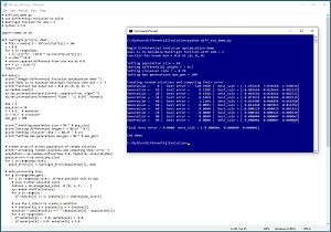 [Click on image for larger view.] Figure 1: Using Differential Evolution Optimization to Solve the Rastrigin Function.
The Rastrigin function with dim = 3 has a known min-value solution of 0.0 at (0, 0, 0). The demo program sets up pop_size = 10 random points where each point is a possible solution. DEO has three key parameters. Differential weight, F, is set to 0.5. Crossover rate, CR, is set to 0.70. Maximum number of generations, max_gen, is set to 100. These parameters will be explained shortly.
The demo program iterates 100 generations. On each generation, each of the 10 possible solution points produces a new candidate solution. If the new candidate solution is better than the current solution that generated the candidate, the new candidate solution replaces the old solution. After 100 generations, the best solution found is at (-0.000001, 0.000000, 0.000001), which is very close to the true solution at (0, 0, 0).
This article assumes you have an intermediate or better familiarity with a C-family programming language. The demo program is implemented using Python, but you should have no trouble refactoring to another language such as C# or JavaScript if you wish.
The complete source code for the demo program is presented in this article and is also available in the accompanying file download. All normal error checking has been removed to keep the main ideas as clear as possible.
To run the demo program, you must have Python installed on your machine. The demo program was developed on Windows 10 using the Anaconda 2020.02 64-bit distribution (which contains Python 3.7.6). The demo program has no significant dependencies so any relatively recent version of Python 3 will work fine.
The Rastrigin Function
The Rastrigin function is a standard benchmark problem for testing optimization algorithms. The Rastrigin function can be defined for dimension = n = 2 or higher. The equation is f(x) = 10n + Sum [ xi^2 - (10 * cos(2*pi*xi^2)) ]. The graph in Figure 2 shows the Rastrigin function for dim = n = 2 where the minimum value is 0.0 at (0, 0). The Rastrigin function is challenging because it resembles an egg carton with many depressions that can trap optimization algorithms into a false local minimum value.
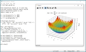 [Click on image for larger view.] Figure 2: The Rastrigin Function for dim = 2.
Understanding Differential Evolution
An evolutionary algorithm is any algorithm that loosely mimics biological evolutionary mechanisms such as mating, chromosome crossover, mutation and natural selection.
A generic form of a standard evolutionary algorithm is:
create a population of possible solutions
loop
  pick two good solutions
  combine them using crossover to create child
  mutate child slightly
  if child is good then
    replace a bad solution with child
  end-if
end-loop
return best solution found
Standard evolutionary algorithms can be implemented using dozens of specific techniques. Differential evolution is a special type of evolutionary algorithm that has a relatively well-defined structure:
create a population of possible solutions
loop
  for-each possible solution
    pick three other random solutions
    combine the three to create a mutation
    combine curr solution with mutation = candidate
    if candidate is better than curr solution then
      replace current solution with candidate
    end-if
  end-for
end-loop
return best solution found
The "differential" term in "differential evolution" is somewhat misleading. Differential evolution does not use Calculus derivatives. The "differential" refers to a specific part of the algorithm where three possible solutions are combined to create a mutation, based on the difference between two of the possible solutions.
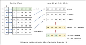 [Click on image for larger view.] Figure 3: One Iteration of Differential Evolution.
The mechanisms of differential evolution are best explained by example. In Figure 3 the goal is to minimize the simple sphere function (rather than the complex Rastrigin function used by the demo program) in dim = 5 which is f(X) = x0^2 + x1^2 + x2^2 + x3^2 + x4^2.
The algorithm creates a population of eight possible solutions. Each initial possible solution is randomly generated. Larger population sizes increase the chance of getting a good result at the expense of computation time. Each possible solution has an associated error. The first possible solution, x[0] = (-3.0, 4.0, 2.0, -5.0, 3.0), has an absolute error of 63.00 because -3.0^2 + 4.0^2 + 2.0^2 + -5.0^2 + 3.0^2 = 9 + 16 + 4 + 25 + 9 = 63.00.
Each of the eight possible solutions is processed one at a time and produces a new candidate solution. First, three of the other possible solutions are randomly selected and labeled a, b, c. In the example, suppose that population items [2], [4] and [6] were randomly selected:
a = (2.0, -1.0,  3.0,  1.0,  -2.0)
b = (3.0,  3.0, -4.0,  1.0,  -2.0)
c = (2.0,  0.0,  5.0,  3.0,  -1.0)
Next, items a, b and c are combined into a mutation y using the equation y = a + F * (b - c). The F is the "differential weight" and is a value between 0 and 2 that must be specified. In the example, F = 0.80.
The calculations for the mutation y are:
(b-c) =  (3.0,  3.0, -4.0,  1.0,  -2.0)
       - (2.0,  0.0,  5.0,  3.0,  -1.0)
      =  (1.0,  3.0, -9.0, -2.0,  -1.0)

F * (b-c) = 0.8 * (1.0,  3.0, -9.0, -2.0,  -1.0)
          = (0.8, 2.4, -7.2, -1.6, -0.8)

a + F * (b - c) =  (2.0, -1.0,  3.0,  1.0, -2.0)
                 + (0.8,  2.4, -7.2, -1.6, -0.8)
                =  (2.8,  1.4, -4.2, -0.6, -2.8)
Next, the mutation y is combined with the current possible solution x[0] using crossover to give a candidate solution. Each cell of the candidate solution takes the corresponding cell value of the mutation with probability CR (usually) or the value of the current possible solution with probability 1-CR (rarely). In the example, CR is set to 0.9 and by chance, the candidate solution took values from the mutation at cells [1], [3], [4] and took values from the current possible solution at cells [0], [2]:
current:   (-3.0, 4.0,  2.0, -5.0,  3.0)
mutation:  ( 2.8, 1.4, -4.2, -0.6, -2.8)

candidate: (-3.0, 1.4,  2.0, -0.6, -2.8)
The last step is to evaluate the newly generated candidate solution. In this example the candidate solution has absolute error = -3.0^2 + 1.4^2 + 2.0^2 + -0.6^2 + -2.8^2 = 9.00 + 1.96 + 4.00 + 0.36 + 7.84 = 23.16. Because the error associated with the candidate solution is less than the error of the current possible solution (63.00), the current possible solution is replaced by the candidate. If the candidate solution had greater error, no replacement would take place.
To summarize, each possible solution in a population creates a new candidate solution. The candidate is generated by combining three randomly selected possible solutions (a mutation) and then combining the mutation with the current possible solution (crossover). The candidate replaces the current solution if the candidate is better (smaller error).
Note that the terminology of differential evolution optimization varies quite a bit from one research paper to another. For example, the possible solutions are sometimes called agents, and the term mutation is used in different ways. And there are many variations of basic differential evolution. For example, in some versions of differential evolution, one cell from the mutation is guaranteed to be used in the candidate.
The Demo Program
The complete demo program, with a few minor edits to save space, is presented in Listing 1.
Listing 1: Differential Evolution Demo Program
# diff_evo_demo.py
# use differential evolution to solve
# Rastrigin function for dim = 3
# Python 3.7.6

import numpy as np

def rastrigin_error(x, dim):
  # f(X) = Sum[xj^2 – 10*cos(2*pi*xj)] + 10n
  z = 0.0
  for j in range(dim):
    z += x[j]**2 - (10.0 * np.cos(2*np.pi*x[j]))
  z += dim * 10.0
  # return squared difference from true min at 0.0
  err = (z - 0.0)**2
  return err

def main():
  print("\nBegin Differential Evolution demo ")
  print("Goal is to minimize Rastrigin dim = 3 ")
  print("Function has known min = 0.0 at (0, 0, 0) ")
  np.random.seed(1)
  np.set_printoptions(precision=6, suppress=True, sign=" ")
  np.set_printoptions(formatter={'float': '{: 0.6f}'.format})

  dim = 3
  pop_size = 10
  F = 0.5   # mutation
  cr = 0.7  # crossover
  max_gen = 100

  print("\nSetting population size = %d " % pop_size)
  print("Setting differential weight F = %0.1f " % F)
  print("Setting crossover rate r = %0.2f " % cr)
  print("Setting max generations max_gen = %d " % max_gen)

  # create array-of-arrays population of random solutions
  print("\nCreating random solutions and their error ")
  population = \
    np.random.uniform(low=-5.0, high=5.0, size=(10,dim))
  popln_errors = np.zeros(pop_size)
  for i in range(pop_size):
    popln_errors[i] = rastrigin_error(population[i], dim)

  # main processing loop
  for g in range(max_gen):
    for i in range(pop_size):  # each possible soln in pop
      # pick 3 other possible solns
      indices = np.arange(pop_size)  # [0, 1, 2, . . ]
      np.random.shuffle(indices)
      for j in range(3):
        if indices[j] == i: indices[j] = indices[pop_size-1]

      # use the 3 others to create a mutation
      a = indices[0]; b = indices[1]; c = indices[2]
      mutation = population[a] + F * \
        (population[b] - population[c])
      for k in range(dim):
        if mutation[k] < -5.0: mutation[k] = -5.0
        if mutation[k] > 5.0: mutation[k] = 5.0

      # use mutation and curr item to create candidate
      new_soln = np.zeros(dim)
      for k in range(dim):
        p = np.random.random()   # between 0.0 and 1.0
        if p < cr:  # usually
          new_soln[k] = mutation[k]
        else:
          new_soln[k] = population[i][k]  # use current

      # replace curr soln if new soln is better
      new_soln_err = rastrigin_error(new_soln, dim)
      if new_soln_err < popln_errors[i]:
        population[i] = new_soln
        popln_errors[i] = new_soln_err

    # find curr best soln
    best_idx = np.argmin(popln_errors)
    best_error = popln_errors[best_idx]
    if g % 10 == 0:
      print("Generation = %4d |  best error = \
%10.4f |  best_soln = " % (g, best_error), end="")
      print(population[best_idx])

  # show final result
  best_idx = np.argmin(popln_errors)
  best_error = popln_errors[best_idx]
  print("\nFinal best error = %0.4f  best_soln = " \
% best_error, end="")
  print(population[best_idx])

  print("\nEnd demo ")

if __name__ == "__main__":
  main()
The demo begins by setting the global NumPy random seed (so results are reproducible) and the key parameters:
np.random.seed(1)
dim = 3
pop_size = 10
F = 0.5   # mutation
cr = 0.7  # crossover
max_gen = 100
Differential evolution optimization is quite sensitive to its parameter values which means you usually must do quite a bit of experimentation to get good results.
The demo creates an initial population of 10 possible solutions and computes the error of each:
population = \
  np.random.uniform(low=-5.0, high=5.0, size=(10,dim))
popln_errors = np.zeros(pop_size)
for i in range(pop_size):
  popln_errors[i] = rastrigin_error(population[i], dim)
In most problems scenarios, you must set limits on the possible values for each element of a solution vector. In this example the range of possible values is set to [-5.0, +5.0].
The main processing loop iterates max_gen times and begins by selecting three random solutions:
for g in range(max_gen):
  for i in range(pop_size):  # each possible soln
    # pick 3 other possible solns
    indices = np.arange(pop_size)  # [0, 1, 2, . . ]
    np.random.shuffle(indices)     # like [6, 0, 5, . .]
    for j in range(3):
      if indices[j] == i:
        indices[j] = indices[pop_size-1]
After picking three random indices, the code checks to see if any of the three are the same as the current population item index i. If so, the duplicate index is arbitrarily replaced by the last of the scrambled index values. Next, items a, b and c are used to create a mutation y using the equation y = a + F * (b - c):
a = indices[0]; b = indices[1]; c = indices[2]
mutation = population[a] + F * \
  (population[b] - population[c])
for k in range(dim):
  if mutation[k] < -5.0: mutation[k] = -5.0
  if mutation[k] > 5.0: mutation[k] = 5.0
If any element of the mutation is outside the range [-5.0, +5.0], it's brought back into range. Next, the current population item and the mutation are combined using crossover to create a new candidate solution:
new_soln = np.zeros(dim)
for k in range(dim):       # each element
  p = np.random.random()   # between 0.0 and 1.0
  if p < cr:  # usually
    new_soln[k] = mutation[k]
  else:
    new_soln[k] = population[i][k]  # use current
There are several alternative strategies for the differential evolution crossover mechanism. For example, the original 1997 research paper ("Differential Evolution - A Simple and Efficient Heuristic for Global Optimization over Continuous Spaces" by R. Storn and K. Price) used a version of contiguous crossover from genetic algorithms. The crossover approach used by the demo is the simplest.
After the new candidate solution has been created, it is compared to the current population item:
# replace curr soln if new soln is better
new_soln_err = rastrigin_error(new_soln, dim)
if new_soln_err < popln_errors[i]:
  population[i] = new_soln
  popln_errors[i] = new_soln_err
Unlike some optimization algorithms, differential evolution doesn't need to explicitly track the best solution found because the best solution will always be in the population. If you modify the basic differential evolution algorithm by periodically replacing a population item with a new randomly generated solution, you need to make sure you don't overwrite the current best solution in the population.
Wrapping Up
Differential evolution optimization was originally designed for use in electrical engineering problems. But DEO has received increased interest as a possible technique for training deep neural networks. The biggest disadvantage of DEO is performance. DEO typically takes much longer to train a deep neural network than standard stochastic gradient descent (SGD) optimization techniques. However, DEO is not subject to the SGD vanishing gradient problem. At some point in the future, it's quite likely that advances in computing power (possibly through quantum computing) will make differential evolution optimization and similar bio-inspired techniques viable alternatives to SGD training techniques.