The Data Science Lab
Logistic Regression from Scratch Using Raw Python
The fundamental technique has been studied for decades, thus creating a huge amount of information and alternate variations that make it hard to tell what is key vs. non-essential information.
Logistic regression is a machine learning technique for binary classification. For example, you might want to predict the sex of a person (male or female) based on their age, state where they live, income and political leaning. There are many other techniques for binary classification, but logistic regression was one of the earliest developed and the technique is considered a fundamental machine learning skill for data scientists.
A good way to see where this article is headed is to take a look at the screenshot in Figure 1. The demo program loads a 200-item set training data and a 40-item set of test data into memory. Next, the demo trains a logistic regression model using raw Python, rather than by using a machine learning code library such as Microsoft ML.NET or scikit.
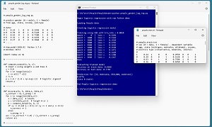 [Click on image for larger view.] Figure 1: Logistic Regression in Action
After training, the model is applied to the training data and the test data. The model scores 86.00 percent accuracy (172 out of 200 correct) on the training data, and 77.50 percent accuracy (31 out of 40 correct) on the test data.
The demo concludes by using the trained model to make a gender prediction for a new, previously unseen person. The new person is age 33, from Nebraska, has an income of $50,000 and is a political moderate. The raw p-value output is 0.0776 and because the p-value is less than 0.5 the prediction is class 0 = male. If the p-value had been greater than 0.5 then the prediction would have been class 1 = female.
This article assumes you have intermediate or better skill with a C-family programming language, but does not assume you know much about logistic regression. The complete source code for the demo program is presented in this article and is also available as an attached download and online.
In order to run the demo program, you'll need to have Python installed on a machine. Installing Python is not trivial, but you can find step-by-step installation instructions here.
The Data
The data is artificial and can be found here. The structure of data looks like:
1   0.24   1   0   0   0.2950   0   0   1
0   0.39   0   0   1   0.5120   0   1   0
1   0.63   0   1   0   0.7580   1   0   0
0   0.36   1   0   0   0.4450   0   1   0
1   0.27   0   1   0   0.2860   0   0   1
. . .
The tab-delimited fields are sex (0 = male, 1 = female), age (divided by 100), state (Michigan = 100, Nebraska = 010, Oklahoma = 001), income (divided by $100,000) and political leaning (conservative = 100, moderate = 010, liberal = 001). For logistic regression, the variable to predict should be encoded as 0 or 1. The numeric predictors should be normalized to all the same range, typically 0.0 to 1.0. The categorical predictors should be one-hot encoded. For example, if there were six states instead of just three, the states would be encoded as 100000, 010000, 001000, 000100, 000010, 000001.
Understanding How Logistic Regression Works
Understanding how logistic regression works is best explained by example. Suppose the goal is to predict the sex of a person who is 35 years old, lives in Michigan, makes $75,000 and who is a political liberal. Each input variable has an associated numeric weight value, and there is a special weight called a bias. Suppose the model weights are [0.3, 0.7, -0.2, 0.1, -0.4, 1.1, 0.6, -0.5] and the bias is 0.9.
The first step is to sum the products of each input variable and its associated weight, and then add the bias:
z = (35)(0.3) + (1)(0.7) + (0)(-0.2) + (0)(0.1) +
    (0.7500)(-0.4) + (0)(1.1) + (0)(0.6) + (1)(-0.5) +
    (0.9)

  = 0.905
The next step is to compute a p-value:
p = 1 / (1 + exp(-z))
  = 1 / (1 + exp(-0.905))
  = 0.7119
The computed p-value will always be between 0 and 1. The last step is to interpret the p-value. If the computed p-value is less than 0.5 the prediction is class 0 (male) and if the computed p-value is greater than 0.5 the prediction is class 1 (female).
Training a Logistic Regression Model
Computing a prediction is simple, but where do the model weights and the bias come from? As it turns out, there are different underlying theoretical models, and each leads to a slightly different way to compute weights from training data. The version that I prefer is based on stochastic gradient descent (SGD) and looks like:
loop through training data:
  get an input vector x[i]
  get target (0 or 1) y
  compute output p using curr wts
  for-each weight:
    wts[j] += lrn_rate * x[j] * (y - p)
  bias += lrn_rate * x[j] * (y - p)
end-loop
The weight update equation is short but is very subtle.
Overall Program Structure
The overall structure of the demo program is presented in Listing 1. The program imports the NumPy library but doesn't import any other external libraries. Most of the control logic is embedded in a main() function. Program-defined function compute_output() is a convenience because it is called many times.
Listing 1: Overall Program Structure
# people_gender_log_reg.py
# Anaconda3-2020.02  Python 3.7.6
# Windows 10/11

import numpy as np

# -----------------------------------------------------------

def compute_output(w, b, x): . . .
def accuracy(w, b, data_x, data_y): . . .
def mse_loss(w, b, data_x, data_y): . . .

# -----------------------------------------------------------

def main():
  # 0. get ready
  print("Begin logistic regression with raw Python demo ")
  np.random.seed(1)

  # 1. load data into memory
  # 2. create model
  # 3. train model
  # 4. evaluate model
  # 5. use model

  print("End People logistic regression demo ")

if __name__ == "__main__":
  main()
The accuracy() function computes classification accuracy, and the mse_loss() function computes how well the model fits the data. The compute_output() function is defined as:
def compute_output(w, b, x):
  z = 0.0
  for i in range(len(w)):
    z += w[i] * x[i]
  z += b
  p = 1.0 / (1.0 + np.exp(-z))  # logistic sigmoid
  return p
The accuracy() function is defined in Listing 2.
Listing 2: The Accuracy Function
def accuracy(w, b, data_x, data_y):
  n_correct = 0; n_wrong = 0
  for i in range(len(data_x)):
    x = data_x[i]  # inputs
    y = int(data_y[i])  # target 0 or 1
    p = compute_output(w, b, x)
    if (y == 0 and p < 0.5) or (y == 1 and p >= 0.5):
      n_correct += 1
    else:
      n_wrong += 1
  acc = (n_correct * 1.0) / (n_correct + n_wrong)
  return acc
The mse_loss() function computes the mean squared error of the model. Its implementation is presented in Listing 3.
Listing 3: The MSE Loss Function
def mse_loss(w, b, data_x, data_y):
  sum = 0.0
  for i in range(len(data_x)):
    x = data_x[i]  # inputs
    y = int(data_y[i])  # target 0 or 1
    p = compute_output(w, b, x)
    sum += (y - p) * (y - p)
  mse = sum / len(data_x)
  return mse
The mse_loss() function is used to monitor training. If the loss value slowly decreases, then training is likely working. A common alternative loss function is cross entropy error.
Loading Data into Memory
The demo program loads the training data using these statements:
  # 1. load data
  print("Loading People data ")
  train_file = ".\\DataLogReg\\people_train.txt"
  train_xy = np.loadtxt(train_file, usecols=range(0,9),
    delimiter="\t", comments="#",  dtype=np.float32)
  train_x = train_xy[:,1:9]
  train_y = train_xy[:,0]
The test data is loaded in the same way:
  test_file = ".\\DataLogReg\\people_test.txt"
  test_xy = np.loadtxt(test_file, usecols=range(0,9),
    delimiter="\t", comments="#", dtype=np.float32)
  test_x = test_xy[:,1:9]
  test_y = test_xy[:,0]
This code assumes that the training and test data are in a subdirectory named DataLogReg. The np.loadtxt() function is just one of several NumPy functions that can be used to load text data from file into memory. The usecols parameter loads columns 0 (the sex variable) through column 8 (the last component of the political type values). After the combined x and y data is stored into a two-dimensional matrix, the data is split into an x matrix (predictors) and a y matrix (target values).
Creating and Training the Model
The code that defines the logistic regression model is:
  # 2. create model
  print("Creating logistic regression model ")
  wts = np.zeros(8)  # one wt per predictor
  lo = -0.01; hi = 0.01
  for i in range(len(wts)):
    wts[i] = (hi - lo) * np.random.random() + lo
  bias = 0.00
Because there are eight predictor values -- age, state (3), income, political-type (3) -- the wts vector has eight cells. Each weight cell is initialized to a random value between -0.01 and +0.01. The model bias is initialized to zero. An alternative design is to place the weights and bias into a Python class.
The code that trains the logistic regression model is presented in Listing 4.
Listing 4: Training the Model
  # 3. train model
  lrn_rate = 0.005
  max_epochs = 10000
  indices = np.arange(len(train_x))  # [0, 1, .. 199]
  print("Training using SGD with lrn_rate = %0.4f " % \
    lrn_rate)
  for epoch in range(max_epochs):
    np.random.shuffle(indices)
    for i in indices:
      x = train_x[i]  # inputs
      y = train_y[i]  # target 0.0 or 1.0
      p = compute_output(wts, bias, x)

      # update all wts and the bias
      for j in range(len(wts)):
        wts[j] += lrn_rate * x[j] * (y - p)
      bias += lrn_rate * (y - p)
    if epoch % 1000 == 0:
      loss = mse_loss(wts, bias, train_x, train_y)
      print("epoch = %5d  |  loss = %9.4f " % \
       (epoch, loss))
  print("Done ")
The learning rate is set to 0.005 and controls how quickly the weights change on each update. The learning rate is a hyperparameter that must be determined by trial and error. The maximum number of training epochs is set to 10,000 and it is also a hyperparameter. If a logistic regression model is trained for too many epochs, the model will overfit, meaning the model will predict very well for the training data, but predict poorly for the test data.
The training code iterates through the training data in a different order on each epoch. A common mistake among beginners is to process the training data without scrambling the order.
Every 1,000 epochs, the training code computes the mean squared error and displays it. In general, training fails more often than it succeeds and so it's important to identify training failure as quickly as possible so that the learning rate and/or maximum number of training epochs can be adjusted.
Evaluating and Using the Trained Model
After training, the demo evaluates the accuracy of the model on the training and test data:
  # 4. evaluate model
  print("Evaluating trained model ")
  acc_train = accuracy(wts, bias, train_x, train_y)
  print("Accuracy on train data: %0.4f " % acc_train)
  acc_test = accuracy(wts, bias, test_x, test_y)
  print("Accuracy on test data: %0.4f " % acc_test)
During training, it's best to evaluate the model using mean squared error. But after training, the ultimate evaluation metric is classification accuracy.
The demo concludes by using the trained model to make a prediction, as shown in Listing 5.
Listing 5: Using the Trained Model
  # 5. use model
  print("Prediction for [33, Nebraska, $50,000, moderate]: ")
  x = np.array([0.33, 0,1,0, 0.5000, 0,1,0], dtype=np.float32)
  p = compute_output(wts, bias, x)
  print("%0.4f " % p)
  if p < 0.5:
    print("class 0 (male) ")
  else:
    print("class 1 (female) ")

  # 6. TODO: save trained weights and bias to file

  print("End People logistic regression demo ")
if __name__ == "__main__":
  main()
Because the model was training using normalized and encoded data, the input must be normalized and encoded in the same way. In most cases the decision threshold is set to 0.5, but for some scenarios the decision threshold can be adjusted up or down.
Wrapping Up
In non-demo scenarios, it's common to compute additional measures of model accuracy: precision, recall and F1 score. These measures of model accuracy are useful when the data is highly skewed towards one class.
One of the major problems for people who are new to logistic regression is that the technique has been studied for decades. This has created a huge amount of information and alternate variations, which makes it difficult to determine what is key information and what is non-essential information.
About the Author
Dr. James McCaffrey works for Microsoft Research in Redmond, Wash. He has worked on several Microsoft products including Azure and Bing. James can be reached at [email protected].