The Data Science Lab
Multinomial Naive Bayes Classification Using the scikit Library
A full-code demo from Dr. James McCaffrey of Microsoft Research shows how to predict the type of a college course by analyzing grade counts for each type of course.
General naive Bayes classification is a classical machine learning technique to predict a discrete value. There are several variations of naive Bayes (NB) including Categorical NB, Bernoulli NB, Gaussian NB and Multinomial NB. The different NB variations are used for different types of predictor data. In Categorical NB the predictor values are strings like "red," "blue" and "green." In Bernoulli NB the predictor values are Boolean/binary like "male" and "female." In Gaussian NB the predictor values are numeric like 27.5 and 13.7.
This article explains Multinomial NB classification where the predictor values are integer counts. Specifically, the raw training data for demo program presented in this article is:
5,7,12,6,4,math
1,6,10,3,0,math
0,9,12,2,1,math
8,8,10,3,2,psychology
7,14,8,0,0,psychology
5,12,9,1,3,psychology
2,16,7,0,2,psychology
3,11,5,4,4,history
5,9,7,4,2,history
8,6,8,0,1,history
Each line represents a college course. The first five values are the number of A grades received by students in the course, the number of B grades, the number of C grades, the number of D grades and the number of F grades. The sixth value on each line is the course type: math, psychology or history. The goal is to predict course type from the counts of each grade. For example, if an unknown course has grade counts of (7,8,7,3,1), what type of course is it?
There are several tools and code libraries that you can use to perform naive Bayes classification. The scikit-learn library (also called scikit or sklearn) is based on the Python language and is one of the most popular machine learning libraries.
A good way to see where this article is headed is to take a look at the screenshot in Figure 1. The demo program begins by loading the synthetic 10-item set training data into memory, where the target labels to predict have been encoded as history = 0, math = 1, psychology = 2. The training data is echoed to the shell.
After the multinomial NB prediction model is created, it is used to predict the course type for the 10 training items. The actual course types and the predicted course types are:
Actual:    1 1 1 2 2 2 2 0 0 0
Predicted: 1 1 1 0 2 2 2 0 0 2
The model accuracy on the training data is 80 percent (8 correct out of 10). The trained model is used to predict the course type for an unknown course with grades distribution of (7, 8, 7, 3, 1). The numeric pseudo-probabilities of the prediction are (0.72, 0.02, 0.26). Because the pseudo-probability at index [0] is the largest, the predicted course type is history.
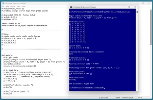 [Click on image for larger view.] Figure 1: Multinomial Naive Bayes Classification Using scikit in Action
This article assumes you have intermediate or better skill with a C-family programming language such as Python or C#, but doesn't assume you know much about naive Bayes classification or the scikit library. The complete source code and data for the demo program are presented in this article. The source code is also available in the accompanying file download and is also online.
Installing the scikit Library
There are several ways to install the scikit library. I recommend installing the Anaconda Python distribution. Anaconda contains a core Python engine plus over 500 libraries that are (mostly) compatible with each other. I used Anaconda3-2020.02, which contains Python 3.7.6 and the scikit 0.22.1 version. The demo code runs on Windows 10 or 11.
Briefly, Anaconda is installed using a Windows self-extracting executable file. The setup process is mostly straightforward and takes about 15 minutes following step-by-step instructions.
There are more up-to-date versions of Anaconda / Python / scikit library available. But because the Python ecosystem has hundreds of libraries, if you install the most recent versions of these libraries, you run a greater risk of library incompatibilities -- a big headache when working with Python.
The Data
When using Multinomial NB, the predictor values are counts. The variable to predict should be zero-based ordinal encoded. For the demo data, history = 0, math = 1, psychology = 2. The encoding is arbitrary but encoding in alphabetical order is a common technique. The resulting training data is:
5,7,12,6,4,1
1,6,10,3,0,1
0,9,12,2,1,1
8,8,10,3,2,2
7,14,8,0,0,2
5,12,9,1,3,2
2,16,7,0,2,2
3,11,5,4,4,0
5,9,7,4,2,0
8,6,8,0,1,0
Encoding the course type values to predict from strings to integers is simple but can be time-consuming for large datasets. The data can be encoded manually, for example by dropping the string data into an Excel spreadsheet and then applying find-replace operations.
It is also possible to programmatically encode string data using the scikit OrdinalEncoder class, or by writing custom code. For example:
fin = open(".\\Data\\college_grades_train_raw.txt", "r")
for line in fin:
  line = line.strip()
  if line.startswith("#"): continue
  tokens = line.split(",")
  if tokens[5] == "history": course = "0"
  elif tokens[5] == "math": course = "1"
  elif tokens[5] == "psychology": course = "2"
  s = tokens[0] + "," + tokens[1] + "," + tokens[2] + "," + \
        tokens[3] + "," + tokens[4] + "," + course + "\n"
  print(s)
fin.close()
As a general rule of thumb, data preparation for machine learning requires roughly 80 percent of the time and effort for creating a prediction model. Based on my experience, this rule of thumb applies to most Multinomial NB scenarios.
Understanding How Multinomial Naive Bayes Classification Works
Understanding how Multinomial naive Bayes classification works is best explained by example. Suppose, as in the demo program, the goal is to predict course type from the counts of each grade received in the course: (7, 8, 7, 3, 1).
There are 78 total students/grades in the three math courses, 117 grades in the four psychology courses, and 77 grades in the three history courses. First, looking only at the counts of the A grades in the training data, there are 5 + 1 + 0 = 6 A grades in the three math courses, or 6 / 78 = 0.0769 A grades. Similarly, there are 22 / 117 = 0.1880 A grades in the psychology courses and there are 16 / 77 = 0.2078 A grades in the history courses.
For the unknown course to predict, there are 7 / 26 = 0.2692 A grades. So, if you had to guess which course type, based only on the A grades, you'd guess history because the 0.2693 frequency of the unknown course is closest to the 0.2078 frequency of A grades in the history courses.
You can repeat this process for the B, C, D and F grades. It turns out that the B grades suggest the unknown course is math, the C grades suggest history, the D grades suggest history, and the F grades suggest psychology. The calculations are shown in Figure 2.
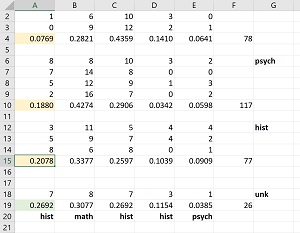 [Click on image for larger view.] Figure 2: Analyzing Each Grade to Predict Course Type
At this point you could use a majority-rule approach and conclude that the unknown course is history because three of the five grade categories suggest history. However, a majority rule doesn't take the strength of each suggestion into account. Multinomial NB combines the suggestions in a mathematically sound way based on probability to make the prediction.
Multinomial NB is called "naive" (meaning unsophisticated) because each predictor count column is analyzed independently, not taking into account interactions between columns. The name "Bayes" refers to Thomas Bayes (1701-1761), a founder of probability theory.
The Demo Program
The complete demo program is presented in Listing 1. I am an unapologetic user of Notepad as my preferred code editor but most of my colleagues use a more sophisticated tool. I indent my Python program using two spaces rather than the more common four spaces.
The program imports the NumPy library which contains numeric array functionality. The MultinomialNB module has the key code for performing Multinomial naive Bayes classification. Notice the name of the root scikit module is sklearn rather than scikit.
Listing 1: Complete Multinomial Naive Bayes Demo Program
# multinomial_bayes.py
# predict college course type from grade counts

# Anaconda3-2020.02  Python 3.7.6
# scikit 0.22.1
# Windows 10/11

import numpy as np
from sklearn.naive_bayes import MultinomialNB

# ---------------------------------------------------------

# Data:
# numAs numBs numCs numDs numFs Course
# history = 0, math = 1, psych = 2
# 5,7,12,6,4,1
# 1,6,10,3,0,1
# . . .

# ---------------------------------------------------------

def main():
  # 0. get ready
  print("\nBegin scikit multinomial Bayes demo ")
  print("Predict (hist = 0, math = 1, psych = 2) from grades ")
  np.random.seed(1)
  np.set_printoptions(precision=4)

  # 1. load data
  train_file = ".\\Data\\college_grades_train.txt"
  XY = np.loadtxt(train_file, usecols=[0,1,2,3,4,5],
    delimiter=",", comments="#", dtype=np.int64)
  X = XY[:,0:5]
  y = XY[:,5]

  print("\nPredictor counts: ")
  print(X)

  print("\nCourse types: ")
  print(y)

  # 2. create and train model
  print("\nCreating multinomial Bayes classifier ")
  model = MultinomialNB(alpha=1)
  model.fit(X, y)
  print("Done ")

  # 3. evaluate model
  y_predicteds = model.predict(X)
  print("\nPredicted classes: ")
  print(y_predicteds)

  acc_train = model.score(X, y)
  print("\nAccuracy on train data = %0.4f " % acc_train)

  # 4. use model
  X = [[7,8,7,3,1]]  # 7 As, 8 Bs, etc.
  print("\nPredicting course for grade counts: "
    + str(X))
  probs = model.predict_proba(X)
  print("\nPrediction probs: ")
  print(probs)

  pred_course = model.predict(X)  # 0,1,2
  courses = ["history", "math", "psychology"]
  print("\nPredicted course: ")
  print(courses[pred_course[0]])

  print("\nEnd multinomial Bayes demo ")

if __name__ == "__main__":
  main()
The demo begins by setting the NumPy random seed:
  # 0. get ready
  print("Begin scikit multinomial Bayes demo ")
  print("Predict (hist = 0, math = 1, psych = 2) from grades ")
  np.random.seed(1)
  np.set_printoptions(precision=4)
. . .
Technically, setting the random seed value isn't necessary, but doing so allows you to get reproducible results in many situations.
Loading the Training and Test Data
The demo program loads the training data into memory using these statements:
  # 1. load data
  train_file = ".\\Data\\college_grades_train.txt"
  XY = np.loadtxt(train_file, usecols=[0,1,2,3,4,5],
    delimiter=",", comments="#", dtype=np.int64)
  X = XY[:,0:5]
  y = XY[:,5]
This code assumes the data files are stored in a directory named Data. There are many ways to load data into memory. I prefer using the NumPy library loadtxt() function but common alternatives are the NumPy genfromtxt() function and the Pandas library read_csv() function.
The demo reads the predictors and the target class labels using a single call to the loadtxt() function. The data is split into a matrix of predictor values and a vector of target values. The colon syntax means "all rows." The demo program does not have any test data, but test data would be read into memory in the same way as the training data.
The demo program prints the 10 predictor count items and the 10 target course type values:
  print("Predictor counts: ")
  print(X)
  print("Course types: ")
  print(y)
In a non-demo scenario with a lot of training data, you might want to display just part of the data.
Creating and Training the Model
Creating and training the naive Bayes classification model is simple:
  # 2. create and train model
  print("Creating multinomial Bayes classifier ")
  model = MultinomialNB(alpha=1)
  model.fit(X, y)
  print("Done ")
Unlike many scikit models, the MultinomialNB class has relatively few (just four) parameters. The constructor signature is:
MultinomialNB(*, alpha=1.0, force_alpha='warn',
  fit_prior=True, class_prior=None)
When working with scikit, you'll spend most of your time reading the documentation and trying to figure out what each model parameter does. The alpha parameter is a bit tricky to explain. Because all forms of naive Bayes compute many frequencies based on counts of data, it's possible for the denominator of a frequency to be zero, which will throw a division-by-zero error. Behind the scenes, the alpha value is added to all counts to eliminate that error. This technique is called Laplacian smoothing. Notice that the default value of alpha is 1.0, so the demo code could have omitted the explicit argument.
The default value of the fit_prior parameter is True. This means that by default the initial relative frequencies of the predictor variable counts are computed based on the data, as shown in Figure 2. If you specify fit_prior=False, then all initial values are assumed to be equal. For example, if there was a course type = chemistry with a total of 100 students, each of the five grades would have an initial frequency of 5 / 100 = 0.0500.
The default value of the class_prior is None. This means that by default the initial relative frequencies of the variable to predict are based on the data, as shown in Figure 2. If you specify initial values for the class_prior parameter, those values will be used instead. For example, setting class_prior = [0.30, 0.40, 0.30] will set the initial relative frequencies of history, math, psychology.
After everything has been prepared, the model is trained using the fit() method. The fit() method has no optional parameters.
Evaluating the Trained Model
The demo computes the accuracy of the trained model like so:
  # 3. evaluate model
  y_predicteds = model.predict(X)
  print("Predicted classes: ")
  print(y_predicteds)
  acc_train = model.score(X, y)
  print("Accuracy on train data = %0.4f " % acc_train)
The score() function computes a simple accuracy, which is just the number of correct predictions divided by the total number of predictions. However, for classification problems you usually want additional evaluation metrics to show how the model predicts for different target labels. For example, if a 10-item dataset had just one math course, eight psychology course and one history course, then a model that predicts psychology for any input would score 80 percent accuracy.
The scikit library has many ways to evaluate a trained prediction model. For scenarios with three or more target class labels, a good technique is to compute and display a confusion matrix:
  from sklearn.metrics import confusion_matrix
  cm = confusion_matrix(y, y_predicteds)  # actual, pred
  print("Confusion matrix raw: ")
  print(cm)
For the demo training data, the output is:
[[2 0 1]
 [0 3 0]
 [1 0 3]]
A raw scikit confusion matrix is difficult to interpret, so I usually implement a program-defined function called show_confusion() that adds basic labels. The output of show_confusion() is:
actual     0: 2 0 1
actual     1: 0 3 0
actual     2: 1 0 3
------------
predicted     0 1 2
You can find the source code for the show_confusion() function here.
Using the Trained Model
The demo program uses the model to predict the course type of a new, previously unseen person:
  # 4. use model
  X = [[7,8,7,3,1]]  # 7 As, 8 Bs, etc.
  print("Predicting course for grade counts: "
    + str(X))
  probs = model.predict_proba(X)
  print("Prediction probs: ")
  print(probs)
Notice the double square brackets on the x-input. The predict_proba() function expects a matrix rather than a vector.
The return result from the predict_proba() function ("probabilities array") is [[0.72 0.02 0.26 ]]. The result has only one row because only one input was supplied. The three values in the row are the pseudo-probabilities of class 0, 1 and 2 respectively.
The demo program concludes with:
pred_course = model.predict(X) # 0,1,2
  courses = ["history", "math", "psychology"]
  print("Predicted course: ")
  print(courses[pred_course[0]])

  # 5. TODO: save model using pickle

  print("End demo ")
The predict() method returns the predicted class, 0, 1, 2, rather than pseudo-probabilities.
Saving the Trained Model
The demo doesn't save the trained model. The most common way to save a trained naive Bayes classifier model is to use the pickle library ("pickle" means to preserve in English). For example:
  import pickle
  print("Saving Multinomial naive Bayes model ")
  path = ".\\Models\\grades_scikit_model.sav"
  pickle.dump(model, open(path, "wb"))
This code assumes there is a directory named Models. The saved model could be loaded and used from another program like so:
  # predict for unknown course
  grade_counts = np.array([[5, 8, 16, 4, 2]], dtype=np.int64)
  with open(path, 'rb') as f:
    loaded_model = pickle.load(f)
  pa = loaded_model.predict_proba(x)
  print(pa)
There are several other ways to save and load a trained scikit model, but using the pickle library is simplest.
Wrapping Up
If you search the internet for an example of a Multinomial naive Bayes classification, you'll find dozens of the exact same example repeated over and over where naive Bayes is used for document classification. For example, the possible document types might be business = 0, crime = 1, finance = 2, politics = 3, science = 4, sports = 5. The predictors are the counts of each word in the English language -- "a," "an," "at," "and" and so on -- in each document. This is an annoyingly huge dataset that obscures what is going on with Multinomial naive Bayes and might give you the impression that Multinomial NB can only be used for document classification, rather than used for many prediction problems where the predictor values are counts.