The Data Science Lab
Gaussian Mixture Model Data Clustering from Scratch Using C#
Data clustering is the process of grouping data items so that similar items are placed in the same cluster. There are several different clustering techniques, and each technique has many variations. Common clustering techniques include k-means, Gaussian mixture model, density-based and spectral. This article explains how to implement Gaussian mixture model (GMM) clustering from scratch using the C# programming language.
Compared to other clustering techniques, GMM clustering gives the pseudo-probabilities of cluster membership, as opposed to just assigning each data item to a single cluster ID. For example, if there are k = 3 clusters, a particular data item might have cluster pseudo-probabilities [0.15, 0.10, 0.85], which indicates the item most likely belongs to cluster ID = 2. However, compared to other techniques, GMM clustering is more complex to implement and a bit more complicated to interpret.
A good way to see where this article is headed is to take a look at the screenshot of a demo program in Figure 1. For simplicity, the demo uses just N = 10 data items:
0.01, 0.10
0.02, 0.09
0.03, 0.10
0.04, 0.06
0.05, 0.06
0.06, 0.05
0.07, 0.05
0.08, 0.01
0.09, 0.02
0.10, 0.01
Each data item is a vector with dim = 2 elements. GMM clustering is designed for strictly numeric data. After GMM with k = 3 clusters is applied to the data, the resulting clustering is: (1, 1, 2, 0, 1, 1, 0, 2, 1, 1). This means data item [0] is assigned to cluster 1, item [1] is assigned to cluster 1, item [2] is assigned to cluster 2, item [3] is assigned to cluster 0 and so on.
Behind the scenes, each of the three clusters has a mean, a 2-by-2 covariance matrix, and a coefficient (sometimes called a weight). The means, covariance matrices and coefficients are used to compute the cluster IDs.
 [Click on image for larger view.] Figure 1: Gaussian Mixture Model Data Clustering in Action
The demo program displays the three cluster means, all of which are [0.550, 0.550]. The three means are the same because there are so few data items. In a non-demo scenario the cluster means will usually be different. GMM clustering is not well-suited for very small or extremely large datasets.
This article assumes you have intermediate or better programming skill but doesn't assume you know anything about Gaussian mixture model clustering. The demo is implemented using C#. Because of the underlying mathematical complexity of GMM, refactoring the demo code to another C-family language is feasible but will require significant effort.
The source code for the demo program is too long to be presented in its entirety in this article. The complete code is available in the accompanying file download. The demo code and data are also available online.
Understanding Gaussian Mixture Model Clustering
One of the keys to GMM clustering is understanding multivariate Gaussian distributions. Suppose you are looking at the heights of a large group of the men. If you create a bar graph of the frequencies of height data it will have a bell-shaped curve with a mean like 68.00 inches and variance (a measure of spread) like 9.00 inches-squared. The total area of the bars will be 1.00.
A Gaussian distribution is a mathematical abstraction where the graph is a smooth curve instead of a collection of bars. A Gaussian distribution is completely characterized by a mean and a variance (or equivalently, a standard deviation which is just the square root of the variance).
The mathematical equation that defines the smooth curve of a Gaussian distribution is called its probability density function (PDF). For one-dimensional (univariate) data, the PDF is:
f(x) = (1 / (s * sqrt(2*pi))) * exp( -1/2 * (x-u)/s)^2 )
where x is the input (like height), u is the mean and s is the standard deviation. For example, if x = 72, u = 68, s = 3, then the PDF is f(x) = (1 / (3 * sqrt(2*pi))) * (exp( -((72 - 68)/(2 * 3))^2 ) = 0.0546.
The PDF value is the height of the bell-shaped curve at the x value. The PDF value can be loosely interpreted as the probability of the corresponding x value.
A multivariate Gaussian distribution extends the ideas. Suppose that instead of looking at just the heights of men, you look at each man's height and weight. So a data item is a vector that looks like (69.50, 170.0) instead of just 69.50. The mean of the multivariate data would be a vector with two values, like (68.00, 175.25).
To describe the spread of the multivariate data, instead of a single variance value, you'd have a 2x2 covariance matrix. If you were looking at data with three values, such as men's (height, weight, age), then the mean of the data would be a vector with three values and the covariance matrix would have a 3x3 shape. Suppose you have a (height, weight, age) covariance matrix like so:
 4.50  7.80  -6.20
 7.80  9.10   5.50
-6.20  5.50   3.60
The three values on the diagonal are variances. The 4.50 at [0][0] is the variance of just the height values. The 9.10 at [1][1] is the variance of just the weight values. The 3.60 at [2][2] is the variance of just the age values.
The value at [0][1] and [1][0] is 7.80, which is the covariance of variable [0] (height) and variable [1] (weight). A covariance is similar to a variance, but covariance is a measure of variability of two variables relative to each other. The value at [0][2] and [2][0] is -6.20 and is the covariance of variable [0] (weight) and variable [2] (age). And the value at [1][2] and [2][1] is the covariance of the weight and ages values. Because a covariance matrix holds both variance values on the diagonal and covariance values on the off-diagonal cells, its real name is a variance-covariance matrix, but that's rather wordy and so the term covariance matrix is generally used.
Computing GMM Pseudo-Probabilities
In GMM clustering, there is one multivariate Gaussian distribution, and one coefficient, for each cluster. So for the two-dimensional demo data with k = 3 clusters, there are three distributions and three coefficients. If you refer to Figure 1 you can see that the values for the first Gaussian distribution are:
mean [0] = [0.0550, 0.0550]

covariance [0] =  0.0002  -0.0001
                 -0.0001   0.0000

coefficient [0] = 0.2017
The values for the second Gaussian distribution are:
mean [1] = [0.0550, 0.0550]

covariance [1] =  0.0011  -0.0011
                 -0.0011   0.0011

coefficient [1] = 0.5859
And the values for the third Gaussian distribution are:
mean [2] = [0.0550, 0.0550]

covariance [2] =  0.0006  -0.0011
                 -0.0011   0.0019

coefficient [2] = 0.2123
These distribution values determine the cluster pseudo-probabilities for a given input x. For the data item [4] = [0.05, 0.06], the cluster pseudo-probabilities are [0.0087, 0.9296, 0.0617]. These are computed in two steps as follows. First, the sum of the distribution PDF values times the coefficients are calculated:
Distribution 0 PDF([0.05, 0.06]) * 0.2017 +
Distribution 1 PDF([0.05, 0.06]) * 0.5859 +
Distribution 2 PDF([0.05, 0.06]) * 0.2123

=   90.7419 * 0.2017 +
  3328.6056 * 0.5859 +
  2098.0352 * 0.2123

= 18.3071 + 1950.2563 + 129.4719

= 2098.0352
Second, the PDF times coefficient values are normalized so that they sum to 1:
pseudo-prob[0] =   18.3071 / 2098.0352 = 0.0087
pseudo-prob[1] = 1950.2563 / 2098.0352 = 0.9296
pseudo-prob[2] =  129.4719 / 2098.0352 = 0.0617
These are the pseudo-probabilities that the item [0.05, 0.06] belongs to cluster 0, cluster 1 and cluster 2.
So, if you have the means, covariance matrices, coefficients and a way to compute the PDF of a distribution, it's relatively easy to compute cluster membership pseudo-probabilities. Somewhat unfortunately, computing all these values is moderately difficult.
Computing a Multivariate Gaussian Distribution PDF Value
One of the major components of implementing GMM clustering from scratch is implementing a function to compute the PDF value for an x value, given the distribution mean and covariance matrix. The math definition for PDF is shown as equation (1) in Figure 2.
Before I go any further, let me point out that if you don't work regularly with machine learning mathematics, the equations might look like a lot of gibberish. But the equations are simpler than they first appear.
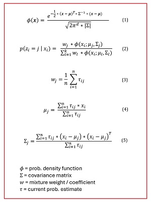 [Click on image for larger view.] Figure 2: The Key Math Equations for GMM Data Clustering
The key symbol in the PDF equation is the Greek uppercase sigma, which represents the covariance matrix. The -1 exponent means the inverse of the matrix. The pair of straight lines means the determinant of the matrix. The inverse and determinant of a covariance matrix are difficult to compute.
Because of the way a covariance matrix is constructed, the most efficient way to compute the inverse and determinant is to use a technique called Cholesky decomposition. Cholesky decomposition is an interesting topic by itself and would take several pages to fully explain. However, it's unlikely that you'll ever have to modify that part of the demo code, so you can consider the inverse and determinant functions as black boxes. See my article "Matrix Inversion Using Cholesky Decomposition With C#" for details.
Computing the Coefficients, Means and Covariance Matrices using EM
Equation (2) in Figure 2 shows how to compute the pseudo-probabilities for a particular data item. The equation corresponds to the worked example presented previously. Fine, but where do the coefficients, means, and covariance matrices come from? The most common meta-algorithm for computing GMM model parameters is called expectation-maximization (EM).
The EM algorithm for GMM data clustering, expressed in very high-level pseudo-code, is:
   loop until very little change in pseudo-probs
      E: use curr coefficients, means, covariances to find probs
      M: use curr probs to update coefficients
         use curr probs to update means
         use curr probs and means to update covariances
    end-loop
    return curr means, covariances, coefficients
In Figure 2, equation (3) shows how to update the coefficients, equation (4) shows how to update the means and equation (5) shows how to update the covariance matrices. If you're a mathematician, you can use the equations to decipher the demo code; if you're a developer, you can use the code to decipher the math equations.
Overall Program Structure
I used Visual Studio 2022 (Community Free Edition) for the demo program. I created a new C# console application and checked the "Place solution and project in the same directory" option. I specified .NET version 6.0. I named the project GaussianMixture. I checked the "Do not use top-level statements" option to avoid the program entry point shortcut syntax.
The demo has no significant .NET dependencies and any relatively recent version of Visual Studio with .NET (Core) or the older .NET Framework will work fine. You can also use the Visual Studio Code program if you like.
After the template code loaded into the editor, I right-clicked on file Program.cs in the Solution Explorer window and renamed the file to the slightly more descriptive GaussianMixtureProgram.cs. I allowed Visual Studio to automatically rename class Program.
The overall program structure is presented in Listing 1. The GaussianMixtureProgram class houses the Main() method, which has all the control logic, and has functions to load data from a text file into memory. The GMM class houses all the Gaussian mixture model clustering functionality. You can see there are a lot of helper methods and functions. All the helpers are relatively simple so the GMM class complexity is due mostly to the interactions and dependencies between the helpers.
Listing 1: Overall Program Structure
using System;
using System.IO;

namespace GaussianMixture
{
  internal class GaussianMixtureProgram
  {
    static void Main(string[] args)
    {
      Console.WriteLine("Begin GMM from scratch C# ");

      // 1. load data into memory
      // 2. instantiate a GMM object
      // 3. use GMM object to cluster the data
      // 4. display clustering results

      Console.WriteLine("End demo ");
      Console.ReadLine();
    } // Main

    static double[][] MatCreate(int rows, int cols) { . . }

    static int NumNonCommentLines(string fn,
      string comment) { . . }

    static double[][] MatLoad(string fn, int[] usecols,
      char sep, string comment) { . . }

    static void MatShow(double[][] m, int dec, int wid) { . . }

    static void VecShow(double[] vec, int dec, int wid,
      bool newLine) { . . }

  } // Program

  public class GMM
  {
    // ------------------------------------------------------

    public int k;  // number clusters
    public int maxIter;
    public Random rnd;  // for initialization
    public int N;  // number data items
    public int dim;  // per data item

    public double[] coefs;
    public double[][] means;  // init'ed by Cluster()
    public double[][][] covars;  // init'ed by Cluster()
    public double[][] probs; // computed clustering probs

    // ------------------------------------------------------

    public GMM(int k, int maxIter, int seed) { . . }

    public int Cluster(double[][] X) { . . }

    public double[] PredictProbs(double[] x) { . . }

    public double[][] PredictProbs(double[][] X) { . . }

    public int[] PredictLabels(double[][] X) { . . }

    private static int ArgMax(double[] vec) { . . }

    private void ExpectStep(double[][] X) { . . }

    private void MaximStep(double[][] X) { . . }

    public double MeanLogLikelihood() { . . }

    static double[][] LocalVecVecScale(double[] x,
      double[] u, double scale) { . . }

    private int[] Select(int N, int n) { . . }

    private void Shuffle(int[] indices) { . . }

    static double LocalMatGaussianPdf(double[] x,
      double[] u, double[][] covar) { . . }

    static double[][] LocalVecToMat(double[] vec,
      int nRows, int nCols) { . . }

    static double[][] LocalMatTranspose(double[][] m) { . . }

    static double[][] LocalMatDiff(double[][] A,
      double[][] B) { . . }

    static double[][] LocalMatProduct(double[][] matA,
      double[][] matB) { . . }

    static double[][] LocalMatCholesky(double[][] m) { . . }

    static double[][]
      LocalMatInverseFromCholesky(double[][] L) { . . }

    static double
      LocalMatDeterminantFromCholesky(double[][] L) { . . }

    static double[][] LocalMatIdentity(int n) { . . }

    static double[][] LocalMatCreate(int rows,
      int cols) { . . }

    static double[][][] LocalMat3DCreate(int factors,
      int rows, int cols) { . . }

    static void LocalMatShow(double[][] m, int dec,
      int wid) { . . }

    static void LocalVecShow(double[] vec, int dec,
      int wid) { . . }

  } // class GMM
} // ns
Loading the Data
The demo program begins by loading the dummy data into memory:
double[][] X = new double[10][];  // 10x2
X[0] = new double[] { 0.01, 0.10 };
X[1] = new double[] { 0.02, 0.09 };
X[2] = new double[] { 0.03, 0.10 };
X[3] = new double[] { 0.04, 0.06 };
X[4] = new double[] { 0.05, 0.06 };
X[5] = new double[] { 0.06, 0.05 };
X[6] = new double[] { 0.07, 0.05 };
X[7] = new double[] { 0.08, 0.01 };
X[8] = new double[] { 0.09, 0.02 };
X[9] = new double[] { 0.10, 0.01 };
For simplicity, the data is hard-coded. In a non-demo scenario, you'll probably want to read the data from a text file into memory using the helper MatLoad() method like so:
string dataFile = "..\\..\\..\\Data\\dummy_10.txt";
double[][] X = MatLoad(dataFile,
  new int[] { 0, 1 }, ',', "#");
The parameters mean to use columns 0 and 1 of the text file, which is comma-delimited, and where the "#" character at the start of a line indicates a comment. The demo program displays the loaded data using the MatShow() function:
Console.WriteLine("Data: ");
MatShow(X, 2, 6);  // 2 decimals, 6 wide
Like most clustering techniques, GMM clustering works best with strictly numeric data that has been normalized so that the magnitudes of all the columns are about the same, typically between 0 and 1, or between -1 and +1. The demo data is normalized so that all the data is between 0.01 and 0.10 because there are so few data points.
Clustering the Data
The GMM clustering object is created and used like so:
int k = 3;  // number of clusters
int mi = 100;  // max iterations
Console.WriteLine("Creating C# scratch" +
  " GMM model k=3, maxIter=100 ");
GMM gmm = new GMM(k, mi, seed: 9);
Console.WriteLine("Clustering ");
int numIter = gmm.Cluster(X);
Console.WriteLine("Done. Used " +
  numIter + " iterations ");
Because GMM clustering is an iterative process, you should specify a maximum number of iterations. This value must be determined by experimentation. The GMM constructor accepts k, the number of clusters to construct, the maximum iterations and a seed value that is used by an internal Random object. The seed value of 9 is used only because it gives representative results. The Random object is used by a helper Shuffle() method, which is used by a helper Select() method, which is used by the primary Cluster() method to initialize the cluster means to k randomly selected data items. Whew!
The data is clustered by calling the Cluster() method. The clustering pseudo-probabilities information is stored internally as a member vector field named probs, which can be accessed by the PredictProbs() method. The Cluster() explicit return value is the number of iterations actually performed in the EM algorithm until the pseudo-probabilities stopped changing very much. Implementing the EM stopping criteria is the primary customization point in the demo program, as you'll see shortly.
Displaying the Clustering Results
The clustering results are displayed like so:
double[][] probs = gmm.PredictProbs(X);
int[] labels = gmm.PredictLabels(X);
Console.WriteLine("Clustering results: ");
for (int i = 0; i < probs.Length; ++i) {
  VecShow(X[i], 2, 6, false);
  Console.Write(" | ");
  VecShow(probs[i], 4, 9, false);
  Console.Write(" | ");
  Console.WriteLine(labels[i]);
}
The PredictProbs() method returns the pseudo-probabilities as an array-of-arrays style matrix. The PredictLabels() method return the clustering as an integer array of 0-based cluster IDs. A cluster ID is just the index of the largest pseudo-probability. The output looks like:
0.01  0.10 |  0.0000   1.0000   0.0000 | 1
0.02  0.09 |  0.0000   1.0000   0.0000 | 1
0.03  0.10 |  0.0000   0.0000   1.0000 | 2
0.04  0.06 |  1.0000   0.0000   0.0000 | 0
0.05  0.06 |  0.0087   0.9296   0.0617 | 1
. . .
The clustering information can be displayed in several ways. For example, instead of displaying by data item, you can display by cluster ID:
for (int cid = 0; cid < 3; ++cid) {
  Console.WriteLine("cid = " + cid);
  for (int i = 0; i < X.Length; ++i) {
    if (labels[i] == cid) {
      for (int j = 0; j < X[i].Length; ++j)
        Console.Write(X[i][j].ToString("F2").PadLeft(6));
      Console.WriteLine("");
    }
  }
}
The output would look like:
cid = 0
  0.04  0.06
  0.07  0.05

cid = 1
  0.01  0.10
  0.02  0.09
. . .
Instead of displaying all clustering information, it's possible to show the clustering pseudo-probabilities for a specific data item:
double[] x = new double[] { 0.05, 0.06 };
double[] p = gmm.PredictProbs(x);
Console.WriteLine("cluster pseudo-probs for" +
  " (0.05, 0.06) = ")
VecShow(p, 4, 9, true);  // add newline
The PredictProbs() method is overloaded to accept either multiple data items as an array-of-arrays matrix, or a single data item as a vector.
The demo program concludes by displaying the means, covariance matrices, and coefficients using these statements:
Console.WriteLine("means: ");
MatShow(gmm.means, 4, 9);
Console.WriteLine("covariances: ");
for (int cid = 0; cid < 3; ++cid)
{
  MatShow(gmm.covars[cid], 4, 9);
  Console.WriteLine("");
}
Console.WriteLine("coefficients: ");
VecShow(gmm.coefs, 4, 9, true);
The MatShow() and VecShow() helper functions make the Main() method a bit cleaner at the expense of yet more helpers.
Customizing the EM Stopping Condition
The demo program implementation stops iterating the expectation-maximization loop using this code:
int iter;
for (iter = 0; iter < this.maxIter; ++iter) {
  double oldMeanLogLike = MeanLogLikelihood();
  this.ExpectStep(X);  // update the probs
  double newMeanLogLike = MeanLogLikelihood();
  if (iter > this.maxIter / 2 &&
    Math.Abs(newMeanLogLike - oldMeanLogLike) < 1.0e-3) {
     break;
  }
  this.MaximStep(X);  // update coefs, means, covars
}
The EM loop stops when the maximum number of iterations has been reached, or if the difference between the average log-likelihood of the pseudo-probabilities is less than 0.001 and the number of iterations is at least half of the maximum number of iterations.
The average log-likelihood is computed by the MeanLogLikelihood() helper method. Suppose the pseudo-probabilities for one data item are (0.10, 0.85, 0.05). The log-likelihood for this item is log(0.10) + log(0.85) + log(0.15) = -2.30 + -0.16 + -2.99 = -5.46. For multiple data items, the average log likelihood is the average of the individual log-likelihood values.
The demo GMM clustering implementation uses minimal change in average log-likelihood as the EM stopping condition mostly because that's the stopping condition used by the scikit-learn library GMM module. In my opinion, this stopping approach is a bit strange because a.) you have to deal with the possibility of log(0), which is negative infinity, and b.) you have to deal with the order of arguments because log-likelihood(x,y,z) = log-likelihood(z,y,x) = log-likelihood(y,x,z) = etc.
There are many other stopping conditions you can implement. One approach I've used is to just directly check to see if the pseudo-probabilities have not changed more than some small epsilon value.
Wrapping Up
It's important to remember that data clustering is an exploratory process. There is no correct clustering of any dataset. In most data clustering scenarios, there should be a human-in-the-loop where human expertise is used to examine clustering results to see if there are any interesting patterns.
Among my colleagues, there are mixed opinions about Gaussian mixture model clustering. Some of my colleagues believe that GMM clustering is arguably the most powerful clustering algorithm. On the other hand, some of my colleagues believe that GMM clustering is an example of an overly complex research solution in search of a problem. I have an intermediate opinion. I think that different clustering techniques -- k-means, density-based, spectral and GMM -- reveal different patterns and that in most scenarios it's not possible to know beforehand which clustering technique is most applicable.