The Data Science Lab
Binary Classification Using PyTorch: Defining a Network
Dr. James McCaffrey of Microsoft Research tackles how to define a network in the second of a series of four articles that present a complete end-to-end production-quality example of binary classification using a PyTorch neural network, including a full Python code sample and data files.
The goal of a binary classification problem is to predict an output value that can be one of just two possible discrete values, such as "male" or "female."
This article is the second in a series of four articles that present a complete end-to-end production-quality example of binary classification using a PyTorch neural network (see the first article about preparing data here).
The example problem is to predict if a banknote (think euro or dollar bill) is authentic or a forgery based on four predictor variables extracted from a digital image of the banknote.
The process of creating a PyTorch neural network binary classifier consists of six steps:
- Prepare the training and test data
- Implement a Dataset object to serve up the data
- Design and implement a neural network
- Write code to train the network
- Write code to evaluate the model (the trained network)
- Write code to save and use the model to make predictions for new previously unseen data
Each of the six steps is fairly complicated, and the six steps are tightly coupled which adds to the difficulty. This article covers the third step.
A good way to see where this series of articles is headed is to take a look at the screenshot of the demo program in Figure 1. The demo begins by creating Dataset and DataLoader objects which have been designed to work with the well-known Banknote Authentication data. Next, the demo creates a 4-(8-8)-1 deep neural network. Then the demo prepares training by setting up a loss function (binary cross entropy), a training optimizer function (stochastic gradient descent), and parameters for training (learning rate and max epochs).
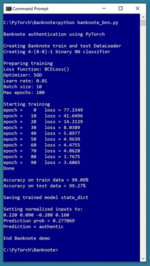 [Click on image for larger view.] Figure 1: Banknote Binary Classification in Action
The demo trains the neural network for 100 epochs using batches of 10 items at a time. An epoch is one complete pass through the training data. For example, if there were 2,000 training data items and training was performed using batches of 50 items at a time, one epoch would consist processing 40 batches of data. During training, the demo computes and displays a measure of the current error. Because error slowly decreases, training is succeeding.
After training the network, the demo program computes the classification accuracy of the model on the training data (99.09 percent correct) and on the test data (99.27 percent correct). Because the two accuracy values are similar, it is likely that model overfitting has not occurred. After evaluating the trained model, the demo program saves the model using the state dictionary approach, which is the most common of three standard techniques.
The demo concludes by using the trained model to make a prediction. The four normalized input predictor values are (0.22, 0.09, -0.28, 0.16). The computed output value is 0.277069 which is less than 0.5 and therefore the prediction is class 0, which in turn means authentic banknote.
This article assumes you have an intermediate or better familiarity with a C-family programming language, preferably Python, but doesn't assume you know very much about PyTorch. The complete source code for the demo program, and the two data files used, are available in the download that accompanies this article. All normal error checking code has been omitted to keep the main ideas as clear as possible.
To run the demo program, you must have Python and PyTorch installed on your machine. The demo programs were developed on Windows 10 using the Anaconda 2020.02 64-bit distribution (which contains Python 3.7.6) and PyTorch version 1.6.0 for CPU installed via pip. You can find detailed step-by-step installation instructions for this configuration in my blog post here.
The Banknote Authentication Data
The raw Banknote Authentication data looks like:
3.6216, 8.6661, -2.8073, -0.44699, 0
4.5459, 8.1674, -2.4586, -1.46210, 0
. . .
-2.5419, -0.65804, 2.6842, 1.1952, 1
The raw data can be found online at banknote authentication Data Set. The goal is to predict the value in the fifth column (0 = authentic banknote, 1 = forged banknote) using the four predictor values. There are a total of 1,372 data items. The raw data was prepared in the following way. First, all four raw numeric predictor values were normalized by dividing by 20 so they're all between -1.0 and +1.0. Next, 1-based ID values from 1 to 1372 were added so that items can be tracked. Next, a utility program split the data into a training data file with 1,097 randomly selected items (80 percent of the 1,372 items) and a test data file with 275 items (the other 20 percent).
After the structure of the training and test files was established, I coded a PyTorch Dataset class to read data into memory and serve the data up in batches using a PyTorch DataLoader object. You can find the article that explains how to create Dataset objects and use them with DataLoader objects here.
The Overall Program Structure
The overall structure of the PyTorch binary classification program, with a few minor edits to save space, is shown in Listing 1. I indent my Python programs using two spaces rather than the more common four spaces as a matter of personal preference.
Listing 1: The Structure of the Demo Program
# banknote_bnn.py
# PyTorch 1.6.0-CPU Anaconda3-2020.02
# Python 3.7.6 Windows 10

import numpy as np
import torch as T
device = T.device("cpu")

# IDs 0001 to 1372 added
# data has been k=20 normalized (all four columns)
# ID  variance  skewness  kurtosis  entropy  class
# [0]    [1]      [2]       [3]       [4]     [5]
#  (0 = authentic, 1 = forgery)  # verified
# train: 1097 items (80%), test: 275 item (20%)

class BanknoteDataset(T.utils.data.Dataset):
  def __init__(self, src_file, num_rows=None): . . .
  def __len__(self): . . .
  def __getitem__(self, idx): . . .

# ----------------------------------------------------

def accuracy(model, ds): . . .

# ----------------------------------------------------

class Net(T.nn.Module):
  def __init__(self): . . .
  def forward(self, x): . . .

# ----------------------------------------------------

def main():
  # 0. get started
  print("Banknote authentication using PyTorch ")

  T.manual_seed(1)
  np.random.seed(1)

  # 1. create Dataset and DataLoader objects
  # 2. create neural network
  # 3. train network
  # 4. evaluate model
  # 5. save model
  # 6. make a prediction

  print("End Banknote demo ")

if __name__== "__main__":
  main()
It's important to document the versions of Python and PyTorch being used because both systems are under continuous development. Dealing with versioning incompatibilities is a significant headache when working with PyTorch and is something you should not underestimate.
I like to use "T" as the top-level alias for the torch package. Most of my colleagues don't use a top-level alias and spell out "torch" dozens of times per program. Also, I use the full form of sub-packages rather than supplying aliases such as "import torch.nn.functional as functional." In my opinion, using the full form is easier to understand and less error-prone than using many aliases.
The demo program defines a program-scope CPU device object. I usually develop my PyTorch programs on a desktop CPU machine. After I get that version working, converting to a CUDA GPU system only requires changing the global device object to T.device("cuda") plus a minor amount of debugging.
The demo program defines just one helper method, accuracy(). All of the rest of the program control logic is contained in a single main() function. It is possible to define other helper functions such as train_net(), evaluate_model(), and save_model(), but in my opinion this modularization approach unexpectedly makes the program more difficult to understand rather than easier to understand.
Defining a Neural Network for Binary Classification
The first step when designing a PyTorch neural network class is to determine its architecture. The number of input nodes is determined by the number of predictor values, four in the case of the Banknote Authentication data. Although there are several design alternatives for the output layer, by far the most common is to use a single output node, where the value of the node is coerced to between 0.0 and 1.0. Then a computed output value that is less than 0.5 corresponds to class 0 (authentic banknote for the demo data) and a computed output value that is greater then 0.5 corresponds to class 1 (forgery). This design assumes that the class-to-predict is encoded as 0 or 1 in the training data, rather than -1 or +1 as is used by some other machine learning binary classification techniques such as averaged perceptron.
The demo network uses two hidden layers, each with eight nodes, resulting in a 4-(8-8)-1 network. The number of hidden layers and the number of nodes in each layer are hyperparameters. Their values must be determined by trial and error guided by experience. The term "AutoML" is sometimes used for any system that programmatically, to some extent, tries to determine good hyperparameter values.
More hidden layers and more hidden nodes is not always better. The Universal Approximation Theorem (sometimes called the Cybenko Theorem) says, loosely, that for any neural architecture with multiple hidden layers, there is an equivalent architecture that has just one hidden layer. For example, a neural network that has two hidden layers with 5 nodes each, is roughly equivalent to a network that has one hidden layer with 25 nodes.
The definition of class Net is shown in Listing 2. In general, most of my colleagues and I use the term "network" or "net" to describe a neural network before it's been trained, and the term "model" to describe a neural network after it's been trained.
Listing 2: Class BanknoteDataset Definition
class Net(T.nn.Module):
  def __init__(self):
    super(Net, self).__init__()
    self.hid1 = T.nn.Linear(4, 8)  # 4-(8-8)-1
    self.hid2 = T.nn.Linear(8, 8)
    self.oupt = T.nn.Linear(8, 1)

    T.nn.init.xavier_uniform_(self.hid1.weight)
    T.nn.init.zeros_(self.hid1.bias)
    T.nn.init.xavier_uniform_(self.hid2.weight)
    T.nn.init.zeros_(self.hid2.bias)
    T.nn.init.xavier_uniform_(self.oupt.weight)
    T.nn.init.zeros_(self.oupt.bias)

  def forward(self, x):
    z = T.tanh(self.hid1(x))
    z = T.tanh(self.hid2(z))
    z = T.sigmoid(self.oupt(z))
    return z
The Net class inherits from torch.nn.Module which provides much of the complex behind-the-scenes functionality. The most common structure for a binary classification network is to define the network layers and their associated weights and biases in the __init__() method, and the input-output computations in the forward() method.
The __init__() Method
The __init__() method begins by defining the demo network's three layers of nodes:
def __init__(self):
    super(Net, self).__init__()
    self.hid1 = T.nn.Linear(4, 8)  # 4-(8-8)-1
    self.hid2 = T.nn.Linear(8, 8)
    self.oupt = T.nn.Linear(8, 1)
The first statement invokes the __init__() constructor method of the Module class from which the Net class is derived. The next three statements define the two hidden layers and the single output layer. Notice that you don't explicitly define an input layer because no processing takes place on the input values.
The Linear() class defines a fully connected network layer. You can loosely think of each of the three layers as three standalone functions (they're actually class objects). Therefore the order in which you define the layers doesn't matter. In other words, defining the three layers in this order:
self.hid2 = T.nn.Linear(8, 8)  # hidden 2
    self.oupt = T.nn.Linear(8, 1)  # output
    self.hid1 = T.nn.Linear(4, 8)  # hidden 1
has no effect on how the network computes its output. However, it makes sense to define the networks layers in the order in which they're used when computing an output value.
The demo program initializes the network's weights and biases like so:
T.nn.init.xavier_uniform_(self.hid1.weight)
    T.nn.init.zeros_(self.hid1.bias)
    T.nn.init.xavier_uniform_(self.hid2.weight)
    T.nn.init.zeros_(self.hid2.bias)
    T.nn.init.xavier_uniform_(self.oupt.weight)
    T.nn.init.zeros_(self.oupt.bias)
If a neural network with one hidden layer has ni input nodes, nh hidden nodes, and no output nodes, there are (ni * nh) weights connecting the input nodes to the hidden nodes, and there are (nh * no) weights connecting the hidden nodes to the output nodes. Each hidden node and each output node has a special weight called a bias, so there'd be (nh + no) biases. For example, a 4-5-3 neural network has (4 * 5) + (5 * 3) = 35 weights and (5 + 3) = 8 biases. Therefore, the demo network has (4 * 8) + (8 * 8) + (8 * 1) = 104 weights and (8 + 8 + 1) = 17 biases.
Each layer has a set of weights which connect it to the previous layer. In other words, self.hid1.weight is a matrix of weights from the input nodes to the nodes in the hid1 layer, self.hid2.weight is a matrix of weights from the hid1 nodes to the hid2 nodes, and self.oupt.weight is a matrix of weights from the hid2 nodes to the output nodes.
It's good practice to explicitly initialize the values of a network's weights and biases, so that your results are reproducible. The demo uses xavier_uniform_() initialization on all weights, and it initializes all biases to 0. The xavier() initialization technique is called glorot() in some neural libraries, notably TensorFlow and Keras. Notice the trailing underscore character in the initializers' names. This indicates the initialization method modifies its weight matrix argument in place by reference, rather than as a return value.
PyTorch 1.6 supports a total of 13 initialization functions, including uniform_(), normal_(), constant_(), and dirac_(). For most binary classification problems, the uniform_() and xavier_uniform_() functions work well.
The uniform_() function requires you to specify a range, for example, the statement:
T.nn.init.uniform_(self.hid1.weight, -0.05, +0.05)
would initialize the hid1 layer weights to random values between -0.05 and +0.05. Although the xavier_uniform_() function was designed for deep neural networks with many layers and many nodes, it usually works well with simple neural networks too, and it has the advantage of not requiring the two range parameters. This is because xavier_uniform_() computes the range values based on the number of nodes in the layer to which it is applied.
With a neural network defined as a class with no parameters as shown, you can instantiate a network object with a single statement:
net = Net().to(device)
Somewhat confusingly for PyTorch beginners, there is an entirely different approach you can use to define and instantiate a neural network. This approach uses the Sequential technique to both define and create a network at the same time. This code creates a neural network that's almost the same as the demo network:
net = T.nn.Sequential(
    T.nn.Linear(4,8),
    T.nn.Tanh(),
    T.nn.Linear(8,8),
    T.nn.Tanh(),
    T.nn.Linear(8,1),
    T.nn.Sigmoid()
  ).to(device)
Notice this approach doesn't use explicit weight and bias initialization so you'd be using whatever the current PyTorch version default initialization scheme is (default initialization has changed at least three times since the PyTorch 0.2 version). It is possible to explicitly apply weight and bias initialization to a Sequential network but the technique is a bit awkward.
When using the Sequential approach, you don't have to define a forward() method because one is automatically created for you. In almost all situations I prefer using the class definition approach over the Sequential technique. The class definition approach is lower level than the Sequential technique which gives you a bit more flexibility. Additionally, understanding the class definition approach is essential if you want to create complex neural architectures such as LSTMs, CNNs, and Transformers.
The forward() Method
When using the class definition technique to define a neural network, you must define a forward() method that accepts input tensor(s) and computes output tensor(s). The demo program's forward() method is defined as:
def forward(self, x):
    z = T.tanh(self.hid1(x))
    z = T.tanh(self.hid2(z))
    z = T.sigmoid(self.oupt(z))
    return z
The x parameter is a batch of one or more tensors. The x input is fed to the hid1 layer and then tanh() activation is applied and the result is returned as a tensor z. The tanh() activation will coerce all hid1 layer node values to be between -1.0 and +1.0. Next, z is fed to the hid2 layer and tanh() is applied. Then the new z tensor is fed to the output layer and logistic sigmoid activation is applied. Logistic sigmoid activation coerces the single output node value to be between 0.0 and 1.0 so that the output value can be loosely interpreted as the probability that the result is class 1.
For binary classifiers, the two most common hidden layer activation functions that I use are the tanh() and relu() functions. The relu() activation function ("rectified linear unit") was designed for use with deep neural networks with many hidden layers, but relu() usually works well with relatively shallow networks too.
A rather annoying characteristic of PyTorch is that there are often multiple variations of the same function. For example, there are at least three tanh() functions: torch.tanh(), torch.nn.Tanh(), and torch.nn.functional.tanh(). Multiple versions of functions exist mostly because PyTorch is an open source project and its code organization evolved somewhat organically over time. There is no good way to deal with the confusion of multiple versions of PyTorch functions. You just have to live with it.
Testing the Network
It's good practice to test a neural network before trying to train it. The short program in Listing 3 shows an example. The test program instantiates a 4-(8-8)-1 neural network as described in this article and then feeds it an input of (0.1, 0.2, 0.3, 0.4). See the screenshot in Figure 2.
Listing 3: Testing the Network
# test_net.py

import torch as T
device = T.device("cpu")

class Net(T.nn.Module):
  def __init__(self):
    super(Net, self).__init__()
    self.hid1 = T.nn.Linear(4, 8)  # 4-(8-8)-1
    self.hid2 = T.nn.Linear(8, 8)
    self.oupt = T.nn.Linear(8, 1)

    T.nn.init.xavier_uniform_(self.hid1.weight)
    T.nn.init.zeros_(self.hid1.bias)
    T.nn.init.xavier_uniform_(self.hid2.weight)
    T.nn.init.zeros_(self.hid2.bias)
    T.nn.init.xavier_uniform_(self.oupt.weight)
    T.nn.init.zeros_(self.oupt.bias)

  def forward(self, x):
    z = T.tanh(self.hid1(x))
    z = T.tanh(self.hid2(z))
    z = T.sigmoid(self.oupt(z))
    return z

print("Begin test ")

T.manual_seed(1)  # for initialization repro
net = Net().to(device)
x = T.tensor([[0.1, 0.2, 0.3, 0.4]],
  dtype=T.float32).to(device)
y = net(x)

print("input = ")
print(x)
print("output = ")
print(y)
print("End test ")
The three key statements in the test program are:
net = Net().to(device)
x = T.tensor([[0.1, 0.2, 0.3, 0.4]],
      dtype=T.float32).to(device)
y = net(x)
The net object is instantiated as you might expect. Notice the input x is a 2-dimensional matrix (indicated by the double square brackets) rather than a 1-dimensional vector because the network is expecting a batch of items as input. You could verify this by setting up a different input like so:
x = T.tensor([[0.1, 0.2, 0.3, 0.4],
              [0.5, 0.6, 0.7, 0.8]],
      dtype=T.float32).to(device)
If you're an experienced programmer but new to PyTorch, the call to the neural network seems to make no sense at all. Where is the forward() method? Why does it look like the net object is being re-instantiated using the x tensor?
As it turns out, the net object inherits a special Python __call__() method from the torch.nn.Module class. Any object that has a __call__() method can invoke the method implicitly using simplified syntax of object(input). Additionally, if a PyTorch object which is derived from Module has a method named forward(), then the __call__() method calls the forward() method. To summarize, the statement y = net(x) invisibly calls the inherited __call__() method which in turn calls the program-defined forward() method. The implicit call mechanism may seem like a major hack but in fact there are good reasons for it.
You can verify the calling mechanism by running this code:
y = net(x)
y = net.forward(x)  # same output
y = net.__call__(x) # same output
In non-exploration scenarios, you should not call a neural network using the __call__() or __forward__() methods because the implied call mechanism does necessary behind-the-scenes logging and other actions.
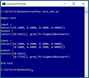 [Click on image for larger view.] Figure 2: Testing the Neural Network
If you look at the screenshot in Figure 2, you'll notice that the first result is displayed as:
output =
tensor([[0.6321]], grad_fn=<SigmoidBackward>)
The grad_fn is the "gradient function" associated with the tensor. A gradient is needed by PyTorch for use in training. In fact, the ability of PyTorch to automatically compute gradients is arguably one of the library's two most important features (along with the ability to compute on GPU hardware). In the demo test program, no training is going on, so PyTorch doesn't need to maintain a gradient on the output tensor. You can optionally instruct PyTorch that no gradient is needed like so:
with T.no_grad():
  y = net(x)
To summarize, when calling a PyTorch neural network to compute output during training, you should never use the no_grad() statement, but when not training, using the no grad() statement is optional but more principled.
Wrapping Up
Defining a PyTorch neural network for binary classification is not trivial but the demo code presented in this article can serve as a template for most scenarios. In situations where a neural network model tends to overfit, you can use a technique called dropout. Model overfitting is characterized by a situation where model accuracy of the training data is good, but model accuracy on the test data is poor.
You can add a dropout layer after any hidden layer. For example, to add two dropout layers to the demo network, you could modify the __init__() method like so:
def __init__(self):
    super(Net, self).__init__()
    self.hid1 = T.nn.Linear(4, 8)  # 4-(8-8)-1
    self.drop1 = T.nn.Dropout(0.50)
    self.hid2 = T.nn.Linear(8, 8)
    self.drop2 = T.nn.Dropout(0.25)
    self.oupt = T.nn.Linear(8, 1)
The first dropout layer will ignore 0.50 (half) of randomly selected nodes in the hid1 layer on each call to forward() during training. The second dropout layer will ignore 0.25 of randomly selected nodes in he hid2 layer during training.
The forward() method would use the dropout layers like so:
def forward(self, x):
    z = T.tanh(self.hid1(x))
    z = self.drop1(z)
    z = T.tanh(self.hid2(z))
    z = self.drop2(z)
    z = T.sigmoid(self.oupt(z))
    return z
Using dropout introduces randomness into the training which tends to make the trained model more resilient to new, previously unseen inputs. Because dropout is intended to control model overfitting, in most situations you define a neural network without dropout, and then add dropout only if overfitting seems to be happening.