The Data Science Lab
Classification Using the scikit k-Nearest Neighbors Module
Dr. James McCaffrey of Microsoft Research uses a full-code, step-by-step demo to predict the species of a wheat seed based on seven predictor variables such as seed length, width and perimeter.
The k-nearest neighbors (k-NN) algorithm is a technique for machine learning classification. The k-NN technique can be used for binary classification (predict where there are exactly two possible values, such as "male" or "female") or for multi-class classification (three or more possible values). A significant limitation of k-NN classification is that all predictor variables must be strictly numeric.
There are several tools and code libraries that you can use to create a k-NN classifier. The scikit-learn library (also called scikit or sklearn) is based on the Python language and is one of the most popular.
A good way to see where this article is headed is to take a look at the screenshot in Figure 1. The demo program uses the scikit k-NN module to create a prediction model for the Wheat Seeds dataset. The goal is to predict the species of a wheat seed (Kama = 0, Rosa = 1, Canadian = 2) based on seven predictor variables such as seed length, width and perimeter.
The demo loads into memory a 180-item set of training data and a 30-item set of test data. Next, the demo creates and trains a k-NN model using the KNeighborsClassifier module from the scikit library.
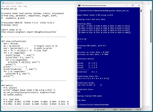 [Click on image for larger view.] Figure 1: Classification Using the scikit k-Nearest Neighbors ModuleE
After training, the model is applied to the training data and the test data. The model scores 96.67 percent accuracy (174 out of 180 correct) on the training data, and 70.00 percent accuracy (21 out of 30 correct) on the test data. The demo computes and displays a confusion matrix for the test data that gives details about which wheat species were incorrectly classified.
The demo concludes by predicting the species of a dummy wheat seed with predictor values of (0.5, 0.5, 0.5, 0.5, 0.5, 0.5, 0.5). The result prediction pseudo-probabilities are [0.71, 0.29 0.00]. Because the value at index [0] is the largest, the predicted species is class 0 = Kama.
This article assumes you have intermediate or better skill with a C-family programming language, but doesn't assume you know much about k-NN classification or the scikit library. The complete source code for the demo program is presented in this article and the accompanying file download. The source code and training and test data are also available online.
Installing the scikit Library
There are several ways to install the scikit library. I recommend installing the Anaconda Python distribution. Anaconda contains a core Python engine plus over 500 libraries that are (mostly) compatible with each other. I used Anaconda3-2020.02 which contains Python 3.7.6 and the scikit 0.22.1 version. The demo code runs on Windows 10 or 11.
Briefly, Anaconda is installed using a Windows self-extracting executable file. The setup process is mostly straightforward and takes about 15 minutes. You can follow step-by-step instructions to help.
There are more up-to-date versions of Anaconda / Python / scikit library available. But because the Python ecosystem has hundreds of libraries, if you install the most recent versions of these libraries, you run a greater risk of library incompatibilities -- a major headache when working with Python.
The Data
The raw Wheat Seeds dataset has 210 items. The source data can be found here. The raw data looks like:
15.26  14.84  0.871   5.763  3.312  2.221  5.22   1
14.88  14.57  0.8811  5.554  3.333  1.018  4.956  1
. . .
17.63  15.98  0.8673  6.191  3.561  4.076  6.06   2
16.84  15.67  0.8623  5.998  3.484  4.675  5.877  2
. . .
11.84  13.21  0.8521  5.175  2.836  3.598  5.044  3
12.3   13.34  0.8684  5.243  2.974  5.637  5.063  3

---------------------------------------------------
10.59  12.41  0.8081  4.899  2.63   0.765  4.519 (min values)
21.18  17.25  0.9183  6.675  4.033  8.456  6.55  (max values)
The first seven values on each line are the numeric predictor variables: seed area, perimeter, compactness, length, width, asymmetry and groove. The last value is the target class label to predict: 1 = Kama, 2 = Rosa, 3 = Canadian.
When using k-NN classification it's important to normalize the numeric predictor values to roughly the same range so that predictor values with large magnitudes don't overwhelm those with small magnitudes. To prepare the data, I dropped it into an Excel spreadsheet. For each predictor column, I computed the min and max values of the column. Then I performed min-max normalization where each value x in a column is normalized to x' = (x - min) / (max - min). The result is that each predictor is a value between 0.0 and 1.0.
I recoded the target class labels from one-based to zero-based. The resulting 210-item dataset looks like:
0.4410  0.5021  0.5708  0.4865  0.4861  0.1893  0.3452  0
0.4051  0.4463  0.6624  0.3688  0.5011  0.0329  0.2152  0
. . .
0.6648  0.7376  0.5372  0.7275  0.6636  0.4305  0.7587  1
0.5902  0.6736  0.4918  0.6188  0.6087  0.5084  0.6686  1
. . .
0.1917  0.2603  0.3630  0.2877  0.2003  0.3304  0.3506  2
0.2049  0.2004  0.8013  0.0980  0.3742  0.2682  0.1531  2
I split the 210-item normalized data into a 180-item training set and a 30-item test set. I used the first 60 items of each target class for training, and the last 10 of each target class for testing.
The Demo Program
The complete demo program is presented in Listing 1. I am not ashamed to admit that Notepad is my preferred code editor, but most of my colleagues prefer something more sophisticated. I indent my Python program using two spaces rather than the more common four spaces.
The program imports the NumPy library, which contains numeric array functionality, and the KNeighborsClassifier module, which contains k-NN classification functionality. Notice the name of the root scikit module is sklearn rather than scikit.
import numpy as np
from sklearn.neighbors import KNeighborsClassifier
In general, it's considered good style to import all the modules that are used in a program at the top of the program rather than at the location where they are used. The demo program uses the "metrics" and "pickle" modules too, so their import statements could have been placed here.
Listing 1: Complete Demo Program
# wheat_knn.py

# predict wheat seed species (0=Kama, 1=Rosa, 2=Canadian)
# from area, perimeter, compactness, length, width,
#   asymmetry, groove

# Anaconda3-2020.02  Python 3.7.6  scikit 0.22.1
# Windows 10/11

import numpy as np
from sklearn.neighbors import KNeighborsClassifier

# ---------------------------------------------------------

def show_confusion(cm):
  dim = len(cm)
  mx = np.max(cm)             # largest count in cm
  wid = len(str(mx)) + 1      # width to print
  fmt = "%" + str(wid) + "d"  # like "%3d"
  for i in range(dim):
    print("actual   ", end="")
    print("%3d:" % i, end="")
    for j in range(dim):
      print(fmt % cm[i][j], end="")
    print("")
  print("------------")
  print("predicted    ", end="")
  for j in range(dim):
    print(fmt % j, end="")
  print("")

# ---------------------------------------------------------

def main():
  # 0. prepare
  print("\nBegin Wheat Seeds k-NN using scikit ")
  np.set_printoptions(precision=4, suppress=True)
  np.random.seed(1)

  # 1. load data
  # 0.4410  0.5021  0.5708  0.4865  0.4861  0.1893  0.3452  0
  # 0.4051  0.4463  0.6624  0.3688  0.5011  0.0329  0.2152  0
  # . . .
  # 0.1917  0.2603  0.3630  0.2877  0.2003  0.3304  0.3506  2
  # 0.2049  0.2004  0.8013  0.0980  0.3742  0.2682  0.1531  2

  print("\nLoading train and test data ")
  train_file = ".\\Data\\wheat_train.txt"  # 180 items
  train_X = np.loadtxt(train_file, usecols=[0,1,2,3,4,5,6],
    delimiter="\t", dtype=np.float32, comments="#")
  train_y = np.loadtxt(train_file, usecols=[7],
    delimiter="\t", dtype=np.int64, comments="#")

  test_file = ".\\Data\\wheat_test.txt"  # 30 items
  test_X = np.loadtxt(test_file, usecols=[0,1,2,3,4,5,6],
    delimiter="\t", dtype=np.float32, comments="#")
  test_y = np.loadtxt(test_file, usecols=[7],
    delimiter="\t", dtype=np.int64, comments="#")

  print("\nTraining data:")
  print(train_X[0:4])
  print(". . . \n")
  print(train_y[0:4])
  print(". . . ")

  # 2. create and train model
  # KNeighborsClassifier(n_neighbors=5, *, weights='uniform',
  #   algorithm='auto', leaf_size=30, p=2, metric='minkowski',
  #   metric_params=None, n_jobs=None)
  # algorithm: 'ball_tree', 'kd_tree', 'brute', 'auto'.

  k = 7
  print("\nCreating kNN model, with k=" + str(k) )
  model = KNeighborsClassifier(n_neighbors=k, algorithm='brute')
  model.fit(train_X, train_y)
  print("Done ")

  # 3. evaluate model
  train_acc = model.score(train_X, train_y)
  test_acc= model.score(test_X, test_y)
  print("\nAccuracy on train data = %0.4f " % train_acc)
  print("Accuracy on test data = %0.4f " % test_acc)

  from sklearn.metrics import confusion_matrix
  y_predicteds = model.predict(test_X)
  cm = confusion_matrix(test_y, y_predicteds)
  print("\nConfusion matrix: \n")
  # print(cm)
  show_confusion(cm)  # custom formatted

  # 4. use model
  X = np.array([[0.5, 0.5, 0.5, 0.5, 0.5, 0.5, 0.5]],
    dtype=np.float32)
  print("\nPredicting class for: ")
  print(X)
  probs = model.predict_proba(X)
  print("\nPrediction probs: ")
  print(probs)

  predicted = model.predict(X)
  print("\nPredicted class: ")
  print(predicted)

  # 5. TODO: save model using pickle

  print("\nEnd demo ")

if __name__ == "__main__":
  main()
All the program logic is contained in a main() function. The demo begins by setting the NumPy random seed:
def main():
  # 0. prepare
  print("Begin Wheat Seeds k-NN using scikit ")
  np.set_printoptions(precision=4, suppress=True)
  np.random.seed(1)
 . . .
Technically, setting the random seed value isn't necessary, but doing so helps you to get reproducible results in most situations. The set_printoptions() function formats NumPy arrays to four decimals without using scientific notation.
Loading the Training and Test Data
The demo program loads the 180-item training data into memory using these statements:
  # 1. load data
  print("Loading train and test data ")
  train_file = ".\\Data\\wheat_train.txt"  # 180 items
  train_X = np.loadtxt(train_file, usecols=[0,1,2,3,4,5,6],
    delimiter="\t", dtype=np.float32, comments="#")
  train_y = np.loadtxt(train_file, usecols=[7],
    delimiter="\t", dtype=np.int64, comments="#")
This code assumes the data files are stored in a directory named Data. There are many ways to load data into memory. I prefer using the NumPy library loadtxt() function, but a common alternative is the Pandas library read_csv() function.
The code reads the training data using two calls to the loadtxt() function, the first for the predictors, the second for the target class labels. An alternative is to read all the data into a NumPy matrix and then split the matrix into a matrix of predictor values and a vector of target labels.
The 30-item test data is read into memory in the same way as the training data:
  test_file = ".\\Data\\wheat_test.txt"  # 30 items
  test_X = np.loadtxt(test_file, usecols=[0,1,2,3,4,5,6],
    delimiter="\t", dtype=np.float32, comments="#")
  test_y = np.loadtxt(test_file, usecols=[7],
    delimiter="\t", dtype=np.int64, comments="#")
The demo program prints the first four predictor items and the first four target politics values:
  print("Training data:")
  print(train_X[0:4])
  print(". . . \n")
  print(train_y[0:4])
  print(". . . ")
In a non-demo scenario you might want to display all the training data and all the test data to verify the data has been read properly.
Understanding k-NN Classification
The k-NN algorithm is arguably the simplest machine learning classification technique. To predict the class label of a data item, the algorithm computes the class labels of the k closest data items and then returns the most common label. For example, suppose you set k = 5 and the five closest items to the item to predict have class labels (2, 1, 0, 1, 1) respectively. Because three of the five closest items are class 1, the predicted class of the item-to-predict is 1.
Because k-NN classification uses a mathematical distance (almost always Euclidean distance) to determine closest neighbors, the data items should be strictly numeric. For example, suppose your data had a predictor variable color with possible values "red," "blue" and "green." There's no obvious way to determine the distance between color values.
Notice that it's possible for k-NN classification to return a tie result. For example, suppose you set k = 9 and the nine closest class labels are (2, 0, 1, 1, 2, 0, 1, 0, 2). There are three of each label. To avoid ties, it's possible to weight the voting procedure by distance to give more importance to closer class labels.
Selecting a value for k in k-NN classification is mostly a matter of trial and error guided by intuition and experience. The common default value for k in most scenarios is k = 5.
Creating the k-NN Prediction Model
The k-NN model is created and trained like so:
  # 2. create and train model
  k = 7
  print("Creating kNN model, with k=" + str(k) )
  model = KNeighborsClassifier(n_neighbors=k, algorithm='brute')
  model.fit(train_X, train_y)
  print("Done ")
The KNeighborsClassifier constructor has eight parameters. The most important is n_neighbors, which is the value of k. The default value is 5. The demo uses 7. The constructor signature is:
KNeighborsClassifier(n_neighbors=5, *, weights='uniform',
  algorithm='auto', leaf_size=30, p=2, metric='minkowski',
  metric_params=None, n_jobs=None)
The possible values for the weights parameter are 'uniform' or 'distance'. The 'uniform' value means that all closest neighbors are used equally, that is, majority-rule voting. The 'distance' value means that voting is weighted so that closest neighbors have more importance.
The possible values for the algorithm parameter are 'auto', 'ball_tree', 'kd_tree' and 'brute'. The 'brute' value means that all possible distances are computed. For example, in the demo data with 180 data items, there are n * (n-1) / 2 = 180 * 179 / 2 = 16,110 distance calculations, which is easily manageable. But for huge datasets, computing all possible distances might not be feasible. The 'ball_tree' and 'kd_tree' parameter values use tree-based algorithms to avoid computing all possible distances, at the expense of accuracy. The default algorithm is 'auto' which uses a wonky decision rule to pick one of the three actual algorithms. I recommend using 'brute', and if your dataset is too large you can try either 'ball_tree' or 'kd_tree'. The leaf_size parameter is used only with the 'ball_tree' and 'kd_tree' values.
The metric and p parameter values determine how k-NN distance is computed. The default values of 'minkowski' and p=2 mean to use Euclidean distance. If you set p=1 then Manhattan distance is used. The metric_params parameter passes arguments to the metric parameter if you pass a custom function. Bottom line: the default values of metric='minkowski' and p=2 are fine in the vast majority of situations.
Evaluating the Trained Model
The demo computes the accuracy of the trained model like so:
  # 3. evaluate model
  train_acc = model.score(train_X, train_y)
  test_acc= model.score(test_X, test_y)
  print("Accuracy on train data = %0.4f " % train_acc)
  print("Accuracy on test data = %0.4f " % test_acc)
The score() function computes a simple accuracy, which is just the number of correct predictions divided by the total number of predictions. However, for multi-class classification problems you usually also want to know the accuracy of the model for each class label. The easiest way to do this is to use the scikit confusion matrix:
  from sklearn.metrics import confusion_matrix
  y_predicteds = net.predict(test_x)
  cm = confusion_matrix(test_y, y_predicteds)
  print("Confusion matrix raw: ")
  print(cm)
For the demo program, the result is:
Confusion matrix raw:
[[5 0 5]
 [3 7 0]
 [1 0 9]]
The raw confusion matrix is a bit difficult to interpret, so I usually write a program-defined helper function to add formatting labels. The code is shown in Listing 2.
Listing 2: Program-Defined Function to Display Confusion Matrix
def show_confusion(cm):
  dim = len(cm)
  mx = np.max(cm)             # largest count in cm
  wid = len(str(mx)) + 1      # width to print
  fmt = "%" + str(wid) + "d"  # like "%3d"
  for i in range(dim):
    print("actual   ", end="")
    print("%3d:" % i, end="")
    for j in range(dim):
      print(fmt % cm[i][j], end="")
    print("")
  print("------------")
  print("predicted    ", end="")
  for j in range(dim):
    print(fmt % j, end="")
  print("")
For the demo program, the output of a show_confusion(cm) call is:
actual     0: 5 0 5
actual     1: 3 7 0
actual     2: 1 0 9
------------
predicted     0 1 2
A good model should have roughly similar accuracy values for all class labels. If any class label has a very low accuracy, you need to investigate. For the demo data, the test accuracy for target class label 0 is only 5 / 10 = 50 percent and should be explored.
Using the Trained Model
The demo uses the trained model like so:
  # 4. use model
  X = np.array([[0.5, 0.5, 0.5, 0.5, 0.5, 0.5, 0.5]],
    dtype=np.float32)
  print("Predicting class for: ")
  print(X)
  probs = model.predict_proba(X)
  print("Prediction probs: ")
  print(probs)
Because the k-NN model was created using normalized data, the X-input must be normalized and encoded in the same way. Notice the double square brackets on the X-input. The predict_proba() method expects a matrix rather than a vector.
The result of the proba() method ("probability array") is a vector of pseudo-probabilities that sum to 1. For k-NN these are the percentages of closest labels. For the demo data with k=7, the result proba vector is [0.71, 0.29, 0.00]. This means that 0.71 * 7 = 5 of the closest neighbors are class 0, and 0.29 * 7 = 2 closest neighbors are class 1, and no closest neighbors are class 2.
The demo concludes by predicting the wheat seed species directly by using the predict() method:
  predicted = model.predict(X)
  print("Predicted class: ")
  print(predicted)
In many scenarios, you want to save the trained model for later use by a different program. The simplest way to save a scikit trained model is to use the pickle library ("pickle" means to preserve in ordinary English). For example:
  import pickle
  print("Saving trained kNN model ")
  path = ".\\Models\\wheat_knn_model.sav"
  pickle.dump(model, open(path, "wb"))
This code assumes there is a subdirectory named Models. The saved model could be loaded into memory and used like this:
  X = np.array([[0.5, 0.5, 0.5, 0.5, 0.5, 0.5, 0.5]],
    dtype=np.int64)
  with open(path, 'rb') as f:
    loaded_model = pickle.load(f)
  pa = loaded_model.predict_proba(x)
  print(pa)
Wrapping Up
The k-NN classification algorithm is often effective, but it's rather primitive. The scikit library has more powerful classification algorithms. The scikit MLPClassifier neural network module can handle complex problems but neural networks require much more training data than k-NN. The scikit DecisionTreeClassifier module can also handle complex problems, but decision trees are highly susceptible to model overfitting.
A common idea is to apply multiple classification algorithms, such as a k-NN, decision tree and neural network, and then combine the results to a final prediction. This is called ensemble learning.