The Data Science Lab
Linear Regression with Pseudo-Inverse Training Using C#
Dr. James McCaffrey presents a complete end-to-end demonstration of linear regression using pseudo-inverse training. Compared to other training techniques, such as stochastic gradient descent, pseudo-inverse training does not require any parameters and so it is especially simple to use.
The goal of a machine learning regression problem is to predict a single numeric value. For example, you might want to predict the bank account balance of an employee based on his age, height, and years of work experience. There are roughly a dozen main regression techniques, including nearest neighbors regression, kernel ridge regression, and neural network regression. Linear regression is the most fundamental technique.
The form of a linear regression prediction equation is y' = (w0 * x0) + (w1 * x1) + . . + (wn * xn) + b where y' is the predicted value, the xi are predictor values, the wi are constants called model weights, and b is a constant called the bias. For example, y' = predicted balance = (-0.54 * age) + (0.38 * height) + (0.11 * experience) + 0.72. Training the model is the process of finding the values of the weights and bias so that predicted y values are close to known correct target y values in a set of training data.
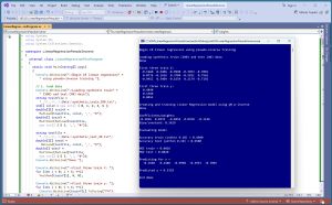 [Click on image for larger view.] Figure 1: Linear Regression with Pseudo-Inverse Training in Action
There are three main techniques to train a linear regression model: stochastic gradient descent (SGD), pseudo-inverse, and closed form training. This article explains how to implement the pseudo-inverse training technique.
A good way to see where this article is headed is to take a look at the screenshot of a demo program in Figure 1. The demo begins by loading a set of synthetic training and test data into memory. The data looks like:
-0.1660,  0.4406, -0.9998, -0.3953, -0.7065,  0.4840
 0.0776, -0.1616,  0.3704, -0.5911,  0.7562,  0.1568
-0.9452,  0.3409, -0.1654,  0.1174, -0.7192,  0.8054
. . .
The first five values on each line are the predictors (sometimes called features). The last value on each line is the target y value to predict. There are 200 training items and 40 test items. Next, the demo trains the linear regression model and then displays the weights and the bias:
Creating and training Linear Regression model using QR p-inverse
Done

Coefficients/weights:
-0.2656  0.0333  -0.0454  0.0358  -0.1146
Bias/constant: 0.3619
Model weights are sometimes called model coefficients. Because there are five predictor variables, there are five weights. Next, the demo evaluates the trained model:
Accuracy train (within 0.10) = 0.4600
Accuracy test (within 0.10) = 0.6500
MSE train = 0.0026
MSE test = 0.0020
For accuracy, a prediction is scored correct if it's within 10% of the true target value. The 10% closeness is arbitrary and a good percentage to use will vary from problem to problem. The accuracy of the model is poor -- just 46% (92 out of 200 correct) on the training data and 65% (25 out of 40 correct) on the training data, because the data has complex, non-linear relations between variables.
The MSE values are mean squared error. They aren't too easy to interpret, other than smaller MSE values are better. They are useful mostly to compare different prediction models. Behind the scenes, linear regression minimizes MSE.
The demo program concludes by using the trained model to make a prediction:
Predicting for x =
  -0.1660   0.4406  -0.9998  -0.3953  -0.7065
Predicted y = 0.5329
The input is the first training item. The predicted y value of 0.5329 is about 11% away from the correct target of 0.4840 and so the prediction would be scored incorrect using the 10% closeness criterion.
This article assumes you have intermediate or better programming skill but doesn't assume you know anything about linear regression. The demo is implemented using C# but you should be able to refactor the demo code to another C-family language if you wish. All normal error checking has been removed to keep the main ideas as clear as possible.
The source code for the demo program is a too long to be presented in its entirety in this article. The complete code and data are available in the accompanying file download, and they're also available online.
The Demo Data
The demo data is synthetic. It was generated by a 5-10-1 neural network with random weights and bias values. The idea here is that the synthetic data does have an underlying, but complex, structure which, in theory, can be predicted.
All of the predictor values are between -1 and +1. There are 200 training data items and 40 test items. With linear regression, it's not necessary to normalize the training data predictor values to the same range because no distance between data items is computed. However, normalizing the predictors doesn't hurt and it's useful just in case you want to send the data to other regression algorithms that require normalization, for example, nearest neighbors regression and kernel ridge regression.
Three common normalization techniques are min-max, z-score, and divide-by-constant. When possible, I recommend using divide-by-constant normalization becasue it's simplest. For example, for a variable that holds employee age values, you could divide all age values by 100 so that the normalized values are all between 0.0 and 1.0.
In practice, linear regression is most often used with data that has strictly numeric predictor variables. But it is possible to use linear regression with categorical data. For categorical data (both ordinal with order, and nominal without order), you can use standard one-hot encoding. For example, for a predictor variable height with possible values (short, medium, tall), you could set short = (1 0 0), medium = (0 1 0), tall = (0 0 1). For binary data, you can use zero-one encoding. For example, for a predictor variable sex, you could set male = 0, female = 1, or vice versa.
Understanding Training Using Pseudo-Inverse
Mathematically, the weight values of a linear regression model can be solved using the equation w = inv(DX) * y, where w is a vector of weights and the bias, DX is a "design matrix", which is a matrix of training predictor data that has a leading column of 1.0 values prepended, inv() is the matrix inverse operation, * means matrix-to-vector multiplication, and y is a vector of the target y values. However, this equation won't work because matrix inverse applies only to square matrices that have the same number of rows and columns, which is almost never the case in machine learning scenarios.
One work-around is to use what's called the Moore-Penrose pseudo-inverse. The math equation is: w = pinv(DX) * y. This technique works because the pseudo-inverse applies to any shape matrix.
The code for pseudo-inverse training is short but a bit deceptive because most of the work is done by helper functions:
public void Train(double[][] trainX, double[] trainY)
{
  int dim = trainX[0].Length; this.weights = new double[dim];
  double[][] X = MatToDesign(trainX);  // design X
  double[][] Xpinv = MatPseudoInv(X); // QR version
  double[] biasAndWts = MatVecProd(Xpinv, trainY);
  this.bias = biasAndWts[0];
  for (int i = 1; i < biasAndWts.Length; ++i)
    this.weights[i - 1] = biasAndWts[i];
}
A design matrix takes the bias into account. For example, if a set of training predictors stored in a matrix X is:
0.50  0.77  0.32
0.92  0.41  0.84
0.64  0.73  0.43
The associated design matrix is:
1.0  0.50  0.77  0.32
1.0  0.92  0.41  0.84
1.0  0.64  0.73  0.43
OK, so all that's needed is a function to compute the pseudo-inverse of a matrix. Unfortunately, implementing a pseudo-inverse function is very difficult. Many mathematicians worked for many years on the problem, and came up with dozens of solutions. The technique used by the demo program is to compute the pseudo-inverse of a matrix using QR decomposition via the Householder algorithm.
The good news is that the demo MatPseudoInv() pseudo-inverse function and its associated MatDecomposeQR() worker function can be considered black boxes. You won't have to modify the code except in very rare situations. The bad news is that because pseudo-inverse is complicated, it can fail due to numerical instability related to arithmetic overflow or underflow. But in practice, pseudo-inverse failure is relatively rare. The chance of failure increases as the size of the set of training data increases. As a crude rule of thumb, closed form pseudo-inverse training for linear regression usually works well when the number of training item is less than 2,000.
For a source matrix A, the QR decomposition is A = Q * R. Taking the inverse of both side of the equation gives inv(A) = inv(Q * R), which simplifies to Ainv = inv(R) * inv(Q). The R matrix is square upper triangular (zeros below the main diagonal) and it's possible to compute the inverse for this special case easily. The inverse of the Q matrix is the transpose of Q (rows and columns switched), which is also easy to compute.
To recap, to train a linear regression model, you can find the pseudo-inverse of the design matrix. To find the pseudo inverse of the design matrix, you can compute the QR decomposition and then easily compute the inverses of the resulting Q and R matrices, and then matrix-multiply those inverses.
An alternative to pseudo-inverse training for linear regression is stochastic gradient descent (SGD) training. Pseudo-inverse training directly finds the values of the weights and the bias that minimize mean squared error. SGD training estimates the values of the weights and bias using an iterative technique that starts with random values, and then slowly adjusts the weights and bias to get closer and closer to the optimal values. SGD requires a learning rate parameter that controls how quickly the values of the weights change, and a maximum iterations parameter that specifies how many iterations to perform. These two parameters must be determined by trial and error.
Unlike SGD training, linear regression pseudo-inverse training does not require any parameters -- it just works -- usually. But pseudo-inverse training is tricky and can sometimes fail, especially with a very large set of training data.
A second alternative to using pseudo-inverse training is closed form training. The equation for closed form training is w = inv(Xt * X) * Xt * y, where X is the design matrix, Xt is its transpose, inv() is regular matrix inverse, * is matrix multiplication, and y is a vector of target values from the training data. Closed form training can fail for large matrices because the Xt * X operation uses many multiplications, and if the matrix values are very small or very large, arithmetic underflow or overflow can occur.
To summarize, there are three ways to train a linear regression model: stochastic gradient descent, pseudo-inverse, closed form. For very large datasets, using SGD is usually the best approach. For medium size datasets, pseudo-inverse often works well. For small datasets, closed from training often works well. Note: There are many other training techniques, such as L-BFGS optimization and simplex optimization, but SGD, pseudo-inverse, and closed form are the most commonly used, at least based on my experience.
The Demo Program
I used Visual Studio 2022 (Community Free Edition) for the demo program. I created a new C# console application and checked the "Place solution and project in the same directory" option. I specified .NET version 8.0. I named the project LinearRegressionPseudoInverse. I checked the "Do not use top-level statements" option to avoid the program entry point shortcut syntax.
The demo has no significant .NET dependencies and any relatively recent version of Visual Studio with .NET (Core) or even the older .NET Framework will work fine. You can also use the Visual Studio Code program if you wish.
After the template code loaded into the editor, I right-clicked on file Program.cs in the Solution Explorer window and renamed the file to the slightly more descriptive LinearRegressionPinvProgram.cs. I allowed Visual Studio to automatically rename class Program.
The overall program structure is presented in Listing 1. All the control logic is in the Main() method in the Program class. The Program class also holds helper functions to load data from file into memory and display data.
All of the linear regression functionality is in a LinearRegressor class. The class exposes a constructor and four methods: Train(), Predict(), Accuracy(), and MSE().
Listing 1: Overall Program Structure
using System;
using System.IO;
using System.Collections.Generic;

namespace LinearRegressionPseudoInverse
{
  internal class LinearRegressionPinvProgram
  {
    static void Main(string[] args)
    {
      Console.WriteLine("Begin C# linear regression" +
        " using pseudo-inverse training ");

      // 1. load data
      // 2. create and train model
      // 3. evaluate model
      // 4. use model to predict

      Console.WriteLine("End demo ");
      Console.ReadLine();
    } // Main()

    static double[][] MatLoad(string fn, int[] usecols,
      char sep, string comment) { . . }

    static double[] MatToVec(double[][] mat) { . . }

    static void VecShow(double[] vec, int dec, int wid) { . . }
  }

  // ========================================================

  public class LinearRegressor
  {
    public double[] weights;
    public double bias;
    private Random rnd;

    public LinearRegressor(int seed = 0) { . . }
    public double Predict(double[] x) { . . }
    public void Train(double[][] trainX, double[] trainY) { . . }
    public double Accuracy(double[][] dataX, double[] dataY,
      double pctClose) { . . }
    public double MSE(double[][] dataX, double[] dataY) { . . }

    // helper functions

    private static double[] MatVecProd(double[][] M,
      double[] v) { . . }

    private static double[][] MatToDesign(double[][] M) { . . }

    private static double[][] MatPseudoInv(double[][] M) { . . }

    private static void MatDecomposeQR(double[][] M,
      out double[][] Q, out double[][] R, bool reduced) { . . }

    private static double[][] MatCopy(double[][] M) { . . }

    private static double[][] MatInverseUpperTri(double[][] U) { . . }

    private static double[][] MatTranspose(double[][] m) { . . }

    private static double[][] MatMake(int nRows, int nCols) { . . }

    private static double[][] MatIdentity(int n) { . . }

    private static double[][] MatProduct(double[][] matA,
      double[][] matB) { . . }

    private static double VecNorm(double[] vec) { . . }

    private static double[][] VecToMat(double[] vec,
        int nRows, int nCols) { . . }

    private static double VecDot(double[] v1, double[] v2) { . . }

  } // class LinearRegressor
} // ns
The demo starts by loading the 200-item training data into memory:
string trainFile = "..\\..\\..\\Data\\synthetic_train_200.txt";
int[] colsX = new int[] { 0, 1, 2, 3, 4 };
double[][] trainX = MatLoad(trainFile, colsX, ',', "#");
double[] trainY = MatToVec(MatLoad(trainFile,
  new int[] { 5 }, ',', "#"));
The training X data is stored into an array-of-arrays style matrix of type double. The data is assumed to be in a directory named Data, which is located in the project root directory. The arguments to the MatLoad() function mean load columns 0, 1, 2, 3, 4 where the data is comma-delimited, and lines beginning with "#" are comments to be ignored. The training y data in column [5] is loaded into a matrix and then converted to a one-dimensional vector using the MatToVec() helper function.
The 40-item test data is loaded into memory using the same pattern that was used to load the training data:
string testFile = "..\\..\\..\\Data\\synthetic_test_40.txt";
double[][] testX = MatLoad(testFile, colsX, ',', "#");
double[] testY = MatToVec(MatLoad(testFile,
  new int[] { 5 }, ',', "#"));
Next, the first three training items are displayed like so:
Console.WriteLine("First three train X: ");
for (int i = 0; i < 3; ++i)
  VecShow(trainX[i], 4, 8);
Console.WriteLine("First three train y: ");
for (int i = 0; i < 3; ++i)
  Console.WriteLine(trainY[i].ToString("F4").PadLeft(8));
In a non-demo scenario, you might want to display all the training and test data to make sure they were loaded correctly.
Creating and Training the Model
The demo creates and trains the model using these statements:
LinearRegressor model = new LinearRegressor();
model.Train(trainX, trainY);
Console.WriteLine("Done ");
Unlike many other regression techniques, the LinearRegressor constructor does not require any arguments. The constructor does have a default seed parameter, set to 0, that is used to instantiate a class Random object. The Random object is not used by the demo implementation, but it's there in case you want to add any randomness to the model. One common idea is to reduce the magnitude of the trained weights by a small random amount, to limit the likelihood of model overfitting.
The Train() method needs only the training data. Because the training algorithm computes the weights and bias values directly, without using an iterative approximation, pseudo-inverse training is sometimes considered a type of closed form training.
After training, the demo displays the model weights and the bias:
Console.WriteLine(Coefficients/weights: ");
for (int i = 0; i < model.weights.Length; ++i)
  Console.Write(model.weights[i].ToString("F4") + "  ");
Console.WriteLine("Bias/constant: " + model.bias.ToString("F4"));
An advantage of linear regression compared to many other regression techniques is that the model is somewhat interpretable. Assuming predictor values have roughly the same range, larger magnitude weights indicate larger importance of the associated predictor variable, and the sign of a weight indicates the direction of a prediction that's created by an increase in the value of the associated predictor variable.
Evaluating the Model
The demo program evaluates the prediction accuracy of the trained model using these statements:
double accTrain = model.Accuracy(trainX, trainY, 0.10);
Console.WriteLine("Accuracy train (within 0.10) = " +
  accTrain.ToString("F4"));
double accTest = model.Accuracy(testX, testY, 0.10);
Console.WriteLine("Accuracy test (within 0.10) = " +
  accTest.ToString("F4"));
The Accuracy() method accepts a percentage-close argument that is used to determine if a prediction is scored as correct or not. This is a minor downside of regression accuracy, but ultimately model accuracy is usually what you're most interested in.
The demo computes the mean squared error for the trained model:
double mseTrain = model.MSE(trainX, trainY);
Console.WriteLine("MSE train = " + mseTrain.ToString("F4"));
double mseTest = model.MSE(testX, testY);
Console.WriteLine("MSE test = " +  mseTest.ToString("F4"));
Mean squared error is the average of the squared differences between predicted y values and the correct target y values in the training data. Smaller MSE values are better. For example, if three predicted y values are 2.5, 5.5, and 3.5 and the associated correct target y values are 2, 8, and 5 then the MSE is ((2.5 - 2)^2 + (5.5 - 8)^2 + (3.5 - 5)^2) / 3 = (0.25 + 6.25 + 2.25) / 3 = 8.75 / 3 = 2.92. If a model make perfect predictions, the MSE would be 0.
In addition to accuracy and MSE, another common model evaluation metric is the coefficient of determination, R2. See Implementing a Coefficient of Determination Function Using C# for details.
Using the Model to Make Predictions
The demo concludes by using the trained model to predict the y value for the first training data item:
double[] x = trainX[0];
Console.WriteLine("Predicting for x = ");
VecShow(x, 4, 9);
double predY = model.Predict(x);
Console.WriteLine("Predicted y = " + predY.ToString("F4"));
The Predict() method just emits the result. An option to consider is adding a verbose parameter to Predict() that, when set to true, displays how the prediction was computed using the model weights and bias.
Wrapping Up
Implementing linear regression using pseudo-inverse training from scratch requires a bit of effort, but it allows you to easily integrate a prediction model with other .NET systems. And a from-scratch implementation also allows you to easily modify the system. For example, you can add error checking that is relevant to your particular problem scenario, or you can add diagnostic WriteLine statements to monitor training.
It's usually not possible to know in advance if a dataset can be modeled well by linear regression. However, it is often a good idea to start with linear regression, because even if it's not effective, linear regression establishes baseline MSE and accuracy results for comparison with more advanced regression techniques such as kernel ridge regression, quadratic regression, and neural network regression.