The Data Science Lab
Classic Stats, Or What ANOVA with R Is All About
New to this type of analysis? It's a classic statistics technique that is still useful. Here's a technique for doing a one-way ANOVA using R.
Analysis of variance (ANOVA) is a classical statistics technique that is used to infer if the means (averages) of three or more groups are all equal, in situations where you only have sample data. If you're new to ANOVA, the name of the technique may be mildly confusing because the goal is to analyze the means of data sets. ANOVA is named as it is because behind the scenes it analyzes variances to make inferences about means.
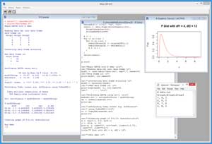
A good way to get an idea of what ANOVA is and to see where this article is headed is to take a look at the screenshot of a demo R session in Figure 1. The source data is stored in a data file named data.txt and has three groups, each of which has four scores.
 [Click on image for larger view.]
Figure 1. ANOVA with R Demo Session
[Click on image for larger view.]
Figure 1. ANOVA with R Demo Session
You can imagine that there are three different English classes at a large high school. Each class is taught using a different strategy and textbook. You want to know if the results are the same or not. You have a test that evaluates students' English ability on a 1-10 scale, but because the test is expensive and time consuming, you can only give the test to four students in each class.
The demo R session begins by reading the sample data into a data frame. You can think of a data frame as a table that can hold both numeric and character data. You can perform ANOVA in R using the built-in aov() function. However, aov() is best used when the source data frame has one observation per row. The demo script calls a program-defined function named myconvert() to create a second data frame that has the correct structure for use by the aov() function.
The demo then calls the aov() function and displays the results. The key value is the one labeled Pr(>F) and which has value 0.00402. This is the probability that all the population means (that is, the true means of all students in the three English classes) are the same. Because this p-value is so small, you'd conclude there's strong evidence that the true means are not all the same, and therefore that the different teaching strategies had some sort of effect.
Next, the demo performs what is called a Tukey honest significance test using the built-in TukeyHSD() function to investigate where the differences in means are. The output compares each pair of groups: G1 vs. G2, G1 vs. G3, and G2 vs. G3. The values in the column labeled "p adj" (for adjusted probability) are the probabilities that each pair of means are the same. In this case, it looks like groups G2 and G3 have different means because the probability that they're equal is 0.0031408, which is very small.
The demo session concludes by generating a graph of the F distribution with degrees of freedom = (4, 12). I'll explain the purpose of this part of the demo shortly.
The Demo Script
The R language can be used interactively or you can place R statements into a text file and execute them as a script. The demo session uses a script.
If you're new to R and want to run the demo script, you need to install R. Installation is quick and easy. Do an Internet search for "Install R" and you'll get a link to an installation page for Windows systems. At the time this article was written, that link was https://cran.r-project.org/bin/windows/base/.
The installation page has a link that points to a self-extracting executable named something like R-3.2.3-win.exe. You can run the installer and accept all the defaults.
To launch the Rgui shell shown in Figure 1, go to directory C:\Program Files\R\R-3.2.3\bin\x64\ and double-click on the Rgui.exe file. To launch a script editor window, click File | New script. Add a comment line and a simple message like:
# AnovaDemo.R
cat("Begin ANOVA with R demo \n\n")
and then go File | Save As and save the script as AnovaDemo.R in any convenient directory. I used C:\AnovaWithR\.
To test your script, call the setwd() and source() functions like so:
> setwd("C:\\AnovaWithR")
> source("AnovaDemo.R")
The overall structure of the demo script is:
# AnovaDemo.R
# function myconvert() defined here
# load data into mydf1 here
# create mydf2 from mydf1 here
# perform ANOVA using aov() here
# perform Tukey HSD here
# create graph here
In the sections that follow, I'll walk you through each statement in the demo script. I assume you have basic scripting and programming knowledge, but I do not assume you know anything about R or ANOVA.
Preparing a Data Frame for ANOVA
The source data is in a text file named data.txt and has contents:
# data.txt
Group1,Group2,Group3
7, 9, 3
6, 9, 5
8, 7, 6
6, 8, 5
This file is saved in directory C:\AnovaWithR\ so it can be accessed directly by the demo script without a path qualifier. The data is loaded into a preliminary data frame named mydf1 using these statements:
cat("Reading data.txt into data frame \n")
mydf1 <- read.table("data.txt", sep=",", header=T)
cat("Data frame is: \n")
print(mydf1, row.names=F)
The built-in read.table() function has many optional parameters. Here, just the token separator (the comma character) and Boolean header flag (T for logical true) parameters are used.
The aov() function cannot use the source data in its original form. The function, like most R statistical functions, expects each data point to be on a single line like this:
Score,Group
7,G1
6,G1
. . .
5,G3
If you're new to R, you should not underestimate the time and effort required for preliminary data massage. In my experience, getting the source data into a suitable format often takes well over 50 percent of my time, and sometimes much more.
One approach to get the data into a correct form is to create a second source data file with the appropriate structure and then call the read.table() function. This is simple and effective. An alternative is to write a program-defined function to generate a new data frame with the desired structure. This is the approach used by the demo script.
At the top of the script, function myconvert() is defined as shown in Listing 1. The function definition begins by determining the number of rows and columns in the source data frame:
myconvert = function(originalDF) {
  nr <- nrow(originalDF)
  nc <- ncol(originalDF)
  tot <- nr * nc
. . .
Next, the function sets up the labels to use and creates a new data frame with the desired properties:
newlabels <- c("G1", "G2", "G3")
result <- data.frame(Score=numeric(tot),
  Group=character(tot), stringsAsFactors=F)
Next, the function loops through the original data frame and populates the result data frame:
k <- 1
for (j in 1:nc) {
  for (i in 1:nr) {
    result$Score[k] <- originalDF[i,j]
    result$Group[k] <- newlabels[j]
    k <- k + 1
  }
}
The custom myconvert() function concludes by returning the new data frame object:
. . .
  return(result)
}
In the body of the demo script, the custom function is called using these statements:
cat("\nConverting data frame structure \n")
mydf2 <- myconvert(mydf1)
cat("\nNew data frame is: \n")
print(head(mydf2, 2), row.names=F)
cat("     . . . \n\n")
Here I print only the first two lines of the new data frame using the head() function, just to save space.
Listing 1: Function to Create Data Frame for ANOVA
myconvert = function(originalDF) {
  nr <- nrow(originalDF) # not inc. header
  nc <- ncol(originalDF)
  tot <- nr * nc

  newlabels <- c("G1", "G2", "G3")
  result <- data.frame(Score=numeric(tot),
    Group=character(tot),
    stringsAsFactors=F)

  k <- 1
  for (j in 1:nc) {
    for (i in 1:nr) {
      result$Score[k] <- originalDF[i,j]
      result$Group[k] <- newlabels[j]
      k <- k + 1
    }
  }
  return(result)
}
Performing ANOVA
Once the source data is in a data frame where each row represents a single data item, performing ANOVA is easy:
cat("Performing ANOVA using aov() \n\n")
mymodel.aov <- aov(mydf2$Score ~ mydf2$Group)
sm <- summary(mymodel.aov)
print(sm)
The aov() function accepts an R formula that looks like:
dataframe$numericCol ~ dataframe$LabelCol
The result is stored into an object named mymodel.aov. In R the '.' character is often used to create more readable function and object names, and the '$' character is used to specify fields of an object.
The output of the ANOVA test is:
            Df Sum Sq Mean Sq F value  Pr(>F)
mydf2$Group  2  24.67  12.333   10.83 0.00402 **
Residuals    9  10.25   1.139
The most important value is the 0.00402, called the p-value, which is the probability that all population means are equal. Because this value is so small, you conclude that the population means are likely not all equal (which isn't quite the same as saying they're all different). The p-value is computed using the value of the F statistic, which for this example is 10.83. A small value of the F statistic indicates all means are the same. The larger the F statistic is, the smaller the p-value is.
The values in the Df column, 2 and 9, are the so-called degrees of freedom. The degrees of freedom are determined by the size and shape of the data. The first value, 2, is the number of groups minus 1. The second value, 9, is the total number of data points minus the number of groups = 12 - 3 = 9.
Performing a Tukey HSD Test
After performing an ANOVA test, if the p-value is small (typically less than 0.05) and you conclude the population means are likely not all equal, you can use the Tukey test to see exactly which means are different.
The demo script performs a Tukey test using these statements:
cat("\nPerforming Tukey honest sig. difference")
cat(" using TukeyHSD()\n\n")
tt <- TukeyHSD(mymodel.aov)
print(tt)
Notice that the TukeyHSD() function accepts the object generated by the aov() function. The "p adj" values in the output are the probabilities that two group means are equal.
Generating an F Distribution Graph
The demo script concludes by generating an example F distribution graph. This isn't a necessary part of an ANOVA analysis; it's done just to illustrate how ANOVA works and how to use the built-in plot() function.
The statements in the script that create the graph are:
x <- seq(0.0, 9.0, by=0.1)
y <- df(x, 4, 12)
plot(x, y, type="l", col="red", ylim=c(0,0.75),
 yaxs="i", ylab="F(x)")
title("F Dist with df1 = 4, df2 = 12")
cat("\nEnd demo \n")
The first statement uses the seq() function to generate a vector of values from 0.0 to 9.0, spaced every 0.1 and stores those values into x. The second statement generates values for an F distribution with 4 and 12 degrees of freedom from the x values using the built-in df() function. Here df() stands for distribution-F rather degrees of freedom.
The shape of an F distribution depends on the two degree of freedom values. Here I use (4, 12) rather than the (2, 9) of the demo data because (4, 12) gives a slightly more representative shape.
For the plot() function, type="l" means line graph. The ylim parameter sets the range of the y-axis. The somewhat cryptic yaxs="i" means to eliminate the small default margin above the x-axis. The ylab parameter sets the label for the y-axis. The title() function adds a title to any graph that is in the current context.
ANOVA Assumptions
An ANOVA test makes three mathematical assumptions. First, the group data items are mathematically independent. Second, the population data sets are distributed normally (as in the Gaussian distribution). Third, the population data sets have equal variances.
There are several built-in R functions that can test these assumptions but interpreting their results is very difficult. The normal distribution assumption can be tested using the mshapiro.test() function. The equality of variances assumption can be tested using the bartlett.test() function.
The problem is that it's highly unlikely that real-world data is exactly normal and has exactly equal variances. And ANOVA still works when data is somewhat non-normal or has non-equal variances. The bottom line is that it's extremely difficult to prove ANOVA assumptions so you must use caution when interpreting results.
ANOVA is closely related to the t-test. The t-test determines if the population means of exactly two groups are equal, in situations where you only have sample data. So, suppose you have three groups, as in the demo. Instead of using ANOVA, you could conceivably perform three t-tests, comparing groups 1 and 2, groups 1 and 3, and groups 2 and 3. However this approach is not recommended because it introduces what is called Type 1 error.
The kind of ANOVA explained in this article is called one-way (or one-factor) ANOVA. There is a different kind of problem called two-way ANOVA. Based on my experience at least, two-way ANOVA is rarely used.
ANOVA is based on the calculated value of an F statistic from a data set. There are other statistical tests that use an F statistic. For example, you can use an F statistic to infer if the variances of two groups of data are the same or not.
About the Author
Dr. James McCaffrey directs the data science and research efforts at Quaetrix, a data analytics company located near Redmond, Washington. Before joining Quaetrix, James was a senior research engineer at Microsoft. James can be reached at [email protected].