The Data Science Lab

Logistic Regression Using R

I predict you'll find this logistic regression example with R to be helpful for gleaning useful information from common binary classification problems.

• By James McCaffrey
• 12/07/2016

Logistic regression is a technique used to make predictions in situations where the item to predict can take one of just two possible values. For example, you might want to predict the credit worthiness ("good" or "bad") of a loan applicant based on their annual income, outstanding debt and so on. Or you might want to predict a person's political party affiliation ("red" or "blue") based on their age, education level, sex and so on. These are sometimes called binary classification problems.

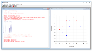
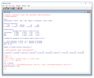
The best way to see where this article is headed is to take a look at the screenshots of a demo R session in Figures 1 and 2. The commands in Figure 1 set up the data for a logistic regression problem where the goal is to predict political party affiliation from age and education level. The commands in Figure 2 use the data to create a prediction model and to make a prediction.

In the sections that follow, I'll walk you through the R commands that generated the output in Figures 1 and 2. After reading this article, you'll have a solid grasp of what type of problem logistic regression solves, know exactly how to perform a logistic regression analysis and understand how to interpret the results of the analysis. All of the R commands for the demo session are presented in this article. You can also get the commands in the accompanying code download.

If you want to follow along with the demo session, and you don't have R installed on your machine, installation (and uninstallation) is quick and easy. Do an Internet search for "install R" and you'll find a URL to a page that has a link to "Download R for Windows." I'm using R version 3.3.1, but by the time you read this article, the current version of R may have changed. If you click on the download link, you'll launch a self-extracting executable installer program. You can accept all the installation option defaults, and R will install in about 30 seconds.

To launch the RGui console program, you can double-click on the shortcut item that will be placed by default on your machine's Desktop. Or, you can navigate to directory C:\Program Files\R\R-3.3.1\bin\x64 and double-click on the Rgui.exe file.

Setting up the Data
In the R Console window, I entered a Ctrl+L command to clear the display. My next two commands were:

> rm(list=ls())
> setwd("C:\\LogisticRegressionUsingR")

The rm function removes all existing objects from memory. The setwd function sets the working directory so that I don't have to fully qualify file names. This command is optional for the demo session because I don't use any files.

My next six commands create the demo data:

> Age <- c(1,5,3,2,6,3,7,4,2,4)
> Edu <- c(4,8,7,5,7,2,5,5,3,7)
> Party <- C("red","red","red","red","red",
+ "blue","blue","blue","blue","blue")
> mydf <- data.frame(Age,Edu,Party)
> mydf$Party <- factor(mydf$Party, levels=c("red","blue"))
> mydf

I use the c function to create three column vectors using hardcoded values for the age, education level and political party for 10 hypothetical people. The "+" sign indicates a statement continuation to the next line. Then I feed the three column vectors to the data.frame function to create a data frame object named mydf.

Here you can think of the age and educational values as being normalized in some way; for example, the age values might represent number of years past age 18, or perhaps actual age divided by 10. I used small numbers just for simplicity.

Even though the values in the Party column of mydf will automatically be interpreted as factor (category) variables, I use the factor function to explicitly define "red" as the first factor and "blue" as the second factor. Notice the return value is assigned back into mydf$Party (the "$" token is used to specify a data frame column).

I display the entire contents of mydf. The output is:

   Age Edu Party
1    1   4   red
2    5   8   red
3    3   7   red
4    2   5   red
5    6   7   red
6    3   2  blue
7    7   5  blue
8    4   5  blue
9    2   3  blue
10   4   7  blue

Notice that R objects use 1-based indexing rather than 0-based indexing. In situations with large data frames you can display just the first few rows by calling head(mydf), or by calling mydf[1:5,] to display the "first 5 rows, all columns."

In most situations you'll want to read data into a data frame from a text file. For example, suppose you had a text file named AgeEduParty.txt with contents:

Age,Edu,Party
1,4,red
5,8,red
...
4,7,blue

You could read the data by calling mydf <- read.table("AgeEduParty.txt", header=T, sep=",") assuming the data file was in the current working directory.

Graphing the Data
After I created the data for a logistic regression analysis, I made a graph of the data using the plot function:

> plot(mydf$Age, mydf$Edu, xlim=c(0,9), ylim=c(0,9),
+ xaxs="i", yaxs="i", col=c("red","blue")[mydf$Party],
+ pch=20, cex=2)

The first two parameters are the values to use for the x and y coordinates. I could've added parameter type="p" to explicitly state that I wanted a points graph, but that's the default type so I omitted the parameter. The xlim and ylim functions specify explicit limits on the axes ranges. Without using xlim and ylim, R would guess at intelligent limit values.

The mysterious looking xaxs="i" and yaxs="i" parameters instruct R to make the lower-left corner of the graph meet at (0, 0). Without these parameters R will add space padding, which I just don't like.

The col parameter specifies the actual colors to use when plotting data points. Here I use "red" and "blue," which correspond to the actual data contents but I could've used "green" and "orange" or any other colors, even though that wouldn't make much sense.

The pch parameter is the "plot character." A value of 21 means a small filled circle. Other possibilities include 22 (filled square) and 24 (filled triangle). The cex is the "character expansion," which here means to double the default size of the circle.

The graph is modified with these three commands:

> axis(side=1, at=c(0:9))
> axis(side=2, at=c(0:9))
> abline(h=0:9,v=0:9, col="gray", lty=3)

In words, the first command means, "for the x-axis, make the axis tick marks 0 through 9 inclusive." Without this command R will guess at tick mark spacing. The second command sets tick marks for the y-axis. The third command displays gray, horizontal and vertical, dashed (lty=3 means line type dashed) grid lines.

Creating the Model
I create and display a logistic regression prediction model with two commands:

> mymodel = glm(Party ~ Age + Edu, data=mydf, family="binomial")
> summary(mymodel)

This means, "Use the general linear model function to create a model that predicts Party from Age and Edu, using the data in mydf, with a logistic regression equation." There's a ton of background theory here, but the glm function is a general-purpose prediction model maker. The family="binomial" parameter creates a logistic regression prediction model. It's actually a shortcut for family=binomial(link="logit").

The summary function displays a lot of information. The key information is in the coefficients section:

Coefficients:
            Estimate Std. Error z value Pr(>|z|)
(Intercept)   3.5566     3.2273   1.102    0.270
Age           0.9939     0.7325   1.357    0.175
Edu          -1.3191     0.8234  -1.602    0.109

The values 3.5566, 0.9939 and -1.3191 define a prediction equation that's best explained by an example. Suppose you want to predict the Party for a person with Age = 1 and Edu = 4. First, you compute an intermediate z-value using the coefficients and input values:

z = 3.5566 + (0.9939)(1) + (-1.3191)(4)
   = -0.7259

And then you compute a p-value:

p = 1 / (1 + e^-z)
   = 1 / (1 + e^(-0.7529))
   = 0.3261

The p-value will always be a value between 0 and 1 and is a probability. If p <= 0.5, the predicted value is the first of the two possible values, "red," in the demo. If p > 0.5, the predicted value is the second possible value, "blue," in the demo. Put another way, p is the probability of the second class (which is a bit counterintuitive).

Notice the output shows a "z value" column. This is a different z from the one used to calculate p. These z values determine the values labeled Pr(>|z|). In greatly simplified terms, these are values that tell you how important each predictor variable is. Smaller values indicate greater significance. In this example, the constant term, the Age variable, and the Edu variable, all have relatively small values (0.270, 0.175, 0.109, respectively) so they all contribute more or less equally to making the prediction equation.

Making Predictions
There are several ways to use a logistic regression model to make a prediction. In the demo I issued the command:

> predict(mymodel, mydf, type="response")

         1          2          3          4 ...
0.32614891 0.11648690 0.06327184 0.25907667 ...

In words, "use mymodel to calculate the prediction probabilities for the 10 data items in mydf." The first data item in mydf is Age = 1 and Edu = 4. The predicted probability is 0.3261, which, because it's less than 0.5 is interpreted as "red." If you examine the output in Figure 2, you'll see that the model predicts 8 out of 10 data items correctly. The model is wrong for data item 5 (actually "red," but incorrectly predicted to be "blue") and 10 (incorrectly predicted to be "red").

Another way to make a prediction is to use the model coefficients directly:

> age <- 1
> edu <- 4
> z <- 3.5566 + (0.9939 * age) + (-1.3191 * edu)
> p <- 1 / (1 + exp(-z))
> p
[1] 0.3260951
> if (p <= 0.5) { cat("predicted party = red \n") }
+ else { cat("predicted party = blue \n") }
predicted party = red

Notice the predicted probability for Age = 1, Edu = 4 of 0.3261 is the same as that returned by the predict function. In this case I copy and pasted the coefficient values. I could've gotten them programmatically like this:

b0 = mymodel$coefficients[[1]]
b1 = mymodel$coefficients[[2]]
b2 = mymodel$coefficients[[3]]
z = b0 + (b1 * 1) + (b2 * 4)
p = 1 / (1 + exp(-z))

The double-bracket indexing is a syntax quirk of R.

A third way to make a prediction is to create a new data frame with the same structure as the one used to create the model (using the with function), but with possibly new data. For example, the commands:

nd = with(mydf, data.frame(Age=1, Edu=4))
nd$pred = predict(mymodel, newdata=nd, type="response")
nd

would display:

  Age Edu      pred
1   1   4 0.3261489

Wrapping Up
In the demo problem, the two predictor variables, Age and Edu, are numeric. Logistic regression can handle categorical predictor variables, too. Similarly, the values to predict "red", "blue" were stored as strings. You can use numeric 0 and 1 if you wish.

Logistic regression is one of the simplest forms of prediction and has several limitations. Logistic regression is used when there are only two possible classes to predict. It is possible to extend logistic regression to handle situations with three or more classes, but in my opinion, there are better approaches than using logistic regression for multinomial classification.

The main drawback to logistic regression is that it can only classify data that are "linearly separable". If you look at the graph in Figure 1, you'll see that no straight line can be drawn that would perfectly separate the red dots and the blue dots. The best you can do is a line that starts at roughly (0, 2) and extends at a 45 degree angle up to about (7, 9). That line will correctly classify 8 out of the 10 data points, which corresponds to what logistic regression does. More powerful techniques such as neural network classification would be able to correctly classify all of the demo data points. In spite of its limitations, logistic regression is a valuable tool for situations in which it's applicable.

• Get Code Download