The Data Science Lab
Neural Network Time Series Regression Using Python
The goal of a time series regression problem is best explained by a concrete example. Suppose you own an airline company and you want to predict the number of passengers you'll have next month based on your historical data. Or maybe you want to forecast your sales amount for the next calendar quarter.
Time series regression problems are usually quite difficult, and there are many different techniques you can use. In this article I'll show you how to do time series regression using a neural network, with "rolling window" data, coded from scratch, using Python.
A good way to see where this article is headed is to take a look at the screenshot in Figure 1 and the graph in Figure 2. The demo program analyzes the number of international airline passengers who travelled each month between January 1949 and December 1960.
 [Click on image for larger view.]
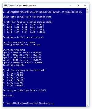
Figure 1. Neural Network Time Series Regression
[Click on image for larger view.]
Figure 1. Neural Network Time Series Regression
The data comes from a benchmark dataset that you can find in many places on the Internet by searching for "airline passengers time series regression." The raw source data looks like:
"1949-01";112
"1949-02";118
"1949-03";132
. . .
"1960-11";390
"1960-12";432
There are 144 data items. The first field is the year and month. The second field is the total number of international airline passengers for the month, in thousands. The demo program creates training data using a rolling window of size 4 to yield 140 training items. The training data is also re-normalized by dividing each passenger count by 100:
(  0)  1.12  1.18  1.32  1.29  1.21
(  1)  1.18  1.32  1.29  1.21  1.35
(  2)  1.32  1.29  1.21  1.35  1.48
(  3)  1.29  1.21  1.35  1.48  1.48
. . .
(139)  6.06  5.08  4.61  3.90  4.32
The first four values on each line are used as predictors. The fifth value is the passenger count to predict. In other words, each set of four consecutive passenger counts is used to predict the next count. The size of the rolling window used here, 4, was determined by trial and error.
The demo creates a neural network with four input nodes, 12 hidden processing nodes, and a single output node. There's just one output node because time series regression predicts just one time unit ahead. The number of hidden nodes in a neural network must be determined by trial and error.
The neural network has (4 * 12) + (12 * 1) = 60 node-to-node weights and (12 + 1) = 13 biases which essentially define the neural network model. Using the rolling window data, the demo program trains the network using the basic stochastic back-propagation algorithm with a learning rate set to 0.01 and a fixed number of iterations set to 10,000. Both the learning rate and number of iterations are free parameters and their values must be determined by experimentation.
The training algorithm uses back-propagation, which is a form of stochastic gradient descent, with a batch size of one item (which is equivalent to "online" training). The error function used is mean squared error because the predicted output value and known correct output value from the training data are numeric. Note that for classification problems, cross entropy error is usually used; cross entropy is not suitable for regression problems.
 [Click on image for larger view.]
Figure 2. Time Series Predicted and Actual Passenger Counts
[Click on image for larger view.]
Figure 2. Time Series Predicted and Actual Passenger Counts
After training is completed, the demo program calculates and displays a few actual passenger counts and passenger counts predicted by the neural model. This data was used to construct the graph in Figure 2.
When performing time series regression, if you want to compute an accuracy metric you must define exactly what it means for a predicted value to be close enough to the actual value to be considered correct. The demo reckons a predicted passenger count value is correct if it is within 10,000 of the actual count. For example, the first normalized actual passenger count is 1.21 meaning 121,000 passengers. In the code, accuracy calculation checks to see if the normalized predicted passenger count, such as 1.33875, is plus or minus 0.10 of the actual normalized count. This corresponds to 0.10 * 100,000 = 10,000 passengers. Using that accuracy criterion, the neural models predicts passenger counts on the 140-item training set with 70.71 percent accuracy, or 99 out of 140 correct.
This article assumes you have intermediate level skill or better with a C-family programming language and a basic knowledge of neural networks. But regardless of your background and experience, you should be able to follow along without too much difficulty.
Program Structure
The demo program is too long to present in its entirety here, but the complete program is available in the accompanying file download. The structure of the demo program, with a few minor edits to save space, is presented in Listing 1. Note that all normal error checking has been removed, and I indent with two space characters rather than the usual four, to save space.
I used Notepad to edit the demo but most of my colleagues prefer one of the many nice Python editors that are available. The demo begins by importing the numpy, random, and math packages. Coding a neural network from scratch allows you to fully understand exactly what's going on, and allows you to experiment with the code. The downside is the extra time and effort required.
Listing 1: Time Series Demo Program Structure
# nn_timeseries.py
# Python 3.x

import numpy as np
import random
import math

def getAirlineData():
  airData = np.zeros(shape=(140,5), dtype=np.float32)
  airData[0] = np.array([1.12, 1.18, 1.32, 1.29, 1.21],
    dtype=np.float32)
  airData[1] = np.array([1.18, 1.32, 1.29, 1.21, 1.35],
    dtype=np.float32)
  # . . .
  airData[139] = np.array([6.06, 5.08, 4.61, 3.90, 4.32],
    dtype=np.float32)
  return airData

def showVector(v, dec): # . . .
def showMatrix(m, dec): # . . .
def showMatrixPartial(m, numRows, dec, indices): # . . .

class NeuralNetwork:  # . . .
def main():
  print("Begin time series with raw Python demo")
  airData = getAirlineData()
  np.set_printoptions(formatter = \
    {'float': '{: 0.2f}'.format})
  print("First four rows of rolling window data: ")
  print(airData[range(0,4),])

  numInput = 4    # rolling window size
  numHidden = 12
  numOutput = 1   # predict next passenger count
  print("\nCreating a %d-%d-%d neural network " %
    (numInput, numHidden, numOutput) )
  nn = NeuralNetwork(numInput, numHidden,
    numOutput, seed=0)

  maxEpochs = 10000
  learnRate = 0.01
  print("Setting maxEpochs = " + str(maxEpochs))
  print("Setting learning rate = %0.3f " % learnRate)
  print("Starting training")
  nn.train(airData, maxEpochs, learnRate)
  print("Training complete ")

  print("First few month-actual-predicted: ")
  acc = nn.accuracy(airData, 0.10)

  print("Accuracy on 140-item data = %0.4f " % acc)
  print("End demo")

if __name__ == "__main__":
  main()

# end script
The demo program hard-codes the training data into a NumPy array-of-array style matrix with 140 rows and 5 columns:
 def getAirlineData():
  airData = np.zeros(shape=(140,5), dtype=np.float32)
  airData[0] = np.array([1.12, 1.18, 1.32, 1.29, 1.21],
    dtype=np.float32)
  airData[1] = np.array([1.18, 1.32, 1.29, 1.21, 1.35],
    dtype=np.float32)
  # . . .
  airData[139] = np.array([6.06, 5.08, 4.61, 3.90, 4.32],
    dtype=np.float32)
  return airData
In a non-demo scenario you'd likely store the data in a text file and then write a helper function to load the data from file into a numpy matrix. The demo loads the data into memory and displays the first few rows:
def main():
  print("Begin time series with raw Python demo")
  airData = getAirlineData()
  np.set_printoptions(formatter = \
    {'float': '{: 0.2f}'.format})
  print("First four rows of rolling window data: ")
  print(airData[range(0,4),])
. . .
Next, the demo creates a neural network using the program-defined NeuralNetwork class:
  numInput = 4    # rolling window size
  numHidden = 12
  numOutput = 1   # predict next passenger count
  print("\nCreating a %d-%d-%d neural network " %
    (numInput, numHidden, numOutput) )
  nn = NeuralNetwork(numInput, numHidden,
    numOutput, seed=0)
The NeuralNetwork constructor accepts a seed value which is passed to a member random number generator. The generator is used to initialize the network's weights and bias values, and to scramble the order in which the data is processed during training. Setting the seed ensures that results are reproducible.
Next, the demo trains the neural network:
  maxEpochs = 10000
  learnRate = 0.01
  print("Setting maxEpochs = " + str(maxEpochs))
  print("Setting learning rate = %0.3f " % learnRate)
  print("Starting training")
  nn.train(airData, maxEpochs, learnRate)
The NeuralNetwork train method uses the back-propagation algorithm which requires a learning rate to control how much the weights and biases change on each update. A too-small learning rate could lead to very slow training, but a too-large learning rate could jump over a good solution. Back-propagation is iterative and requires a stopping condition, in this case, a maximum number of iterations. Iterating too many times could lead to over-fitting, a situation where the model predicts very well on the training data, but predicts poorly on new, previously unseen data.
During training, the mean squared error of the neural network, using the current weights and biases, is displayed every 2,000 iterations. Error is somewhat difficult to interpret, but it's important to observe error so you can quickly catch situations where error is not decreasing.
The demo concludes by calculating and displaying a custom prediction accuracy metric:
. . .
  print("Training complete ")
  print("First few month-actual-predicted: ")
  acc = nn.accuracy(airData, 0.10)
  print("Accuracy on 140-item data = %0.4f " % acc)
  print("End demo")
if __name__ == "__main__":
  main()
The second argument passed to the accuracy method, 0.10, is an absolute value meaning a predicted count is considered correct that count is plus or minus 0.10 of the actual (normalized) count. An alternative approach is to code the accuracy method so that the second parameter is interpreted as a percentage. For example, a value of 0.10 means a predicted count is correct if it is between 0.90 times the actual count, and 1.10 times the count.
Regression vs. Classification
The NeuralNetwork class definition contains a computeOutputs method. The key difference between a neural network that performs regression, and one that performs classification, is how the output nodes are computed. The code for method computeOutputs begins with:
def computeOutputs(self, xValues):
  hSums = np.zeros(shape=[self.nh], dtype=np.float32)
  oSums = np.zeros(shape=[self.no], dtype=np.float32)
. . .
Here local arrays hSums and oSums are scratch arrays that hold the pre-activation sum of products for the hidden nodes and the output nodes respectively. The NumPy zeros function accepts a shape argument that determines the dimensions of the array. The shape value can be a list as shown, or a tuple, or a scalar value.
Next, the pre-activation sums of products for the hidden nodes are computed:
  for i in range(self.ni):
    self.iNodes[i] = xValues[i]

  for j in range(self.nh):
    for i in range(self.ni):
      hSums[j] += self.iNodes[i] * self.ihWeights[i,j]

  for j in range(self.nh):
    hSums[j] += self.hBiases[j]
Here the bias values are added in a separate for-loop. You could improve efficiency slightly, at the expense of clarity, by adding the bias values in the previous loop, but any performance gain would be tiny.
Next, the hidden node values are computed by applying the activation function:
  for j in range(self.nh):
    self.hNodes[j] = self.hypertan(hSums[j])
The demo uses a program defined hyperbolic tangent static function, which is essentially a wrapper around the built-in Python math.tanh function. The hidden node activation function is hard-coded. For time series regression, an alternative to using tanh is to use the logistic sigmoid function.
Next, the pre-activation output node value is computed:
  for k in range(self.no):
    for j in range(self.nh):
      oSums[k] += self.hNodes[j] * self.hoWeights[j,k]

  for k in range(self.no):
    oSums[k] += self.oBiases[k]
At this point, a neural network classifier would apply softmax activation to the output nodes. However, for neural network regression, no activation is applied. Using no activation is sometimes called identity activation. Note that there is just a single output node so the demo code could have ben refactored so that the hNodes object is a single variable rather than an array.
Method computeOutputrs concludes by transferring the values in the oSums scratch array to the oNodes neural network array:
. . .
  self.oNodes = oSums  # "Identity activation"

  result = np.zeros(shape=self.no, dtype=np.float32)
  for k in range(self.no):
    result[k] = self.oNodes[k]

  return result
The output node value is copied into a local array and returned. This is mostly for calling convenience.
Wrapping Up
The demo program creates a time series regression model but doesn't make a prediction. The last training data item is (6.06, 5.08, 4.61, 3.90, 4.32). To make a prediction for January 1961, the first time step beyond the training data, you'd simply pass (5.08, 4.61, 3.90, 4.32) to method computeOutputs in the trained network.
If you wanted to, you could then take that output value, append it to (4.61, 3.90, 4.32) and then make a prediction for the next time step. You could repeat this process as many times as you wish. This process is called extrapolation. However, the further away you get from the training data, the less accurate your predictions will be.
About the Author
Dr. James McCaffrey works for Microsoft Research in Redmond, Wash. He has worked on several Microsoft products including Azure and Bing. James can be reached at [email protected].