The Data Science Lab
Data Prep for Machine Learning: Outliers
After previously detailing how to examine data files and how to identify and deal with missing data, Dr. James McCaffrey of Microsoft Research now uses a full code sample and step-by-step directions to deal with outlier data.
This article explains how to programmatically identify and deal with outlier data (it's a follow-up to "Data Prep for Machine Learning: Missing Data"). Suppose you have a data file of loan applications. Examples of outlier data include a person's age of 99 (either a very old applicant or possibly a placeholder value that was never changed) and a person's country of "Cannada" (probably a transcription error).
In situations where the source data file is small, about 500 lines or less, you can usually find and deal with outlier data manually. But in almost all realistic scenarios with large datasets you must handle outlier data programmatically.
Preparing data for use in a machine learning (ML) system is time consuming, tedious, and error prone. A reasonable rule of thumb is that data preparation requires at least 80 percent of the total time needed to create an ML system. There are three main phases of data preparation: cleaning, normalizing and encoding, and splitting. Each of the three phases has several steps. Dealing with outlier data is part of the data cleaning phase.
A good way to understand outlier data and see where this article is headed is to take a look at the screenshot of a demo program in Figure 1. The demo uses a small text file where each line represents an employee. The demo analyzes a representative numeric column (age) and then analyzes a representative categorical column (region).
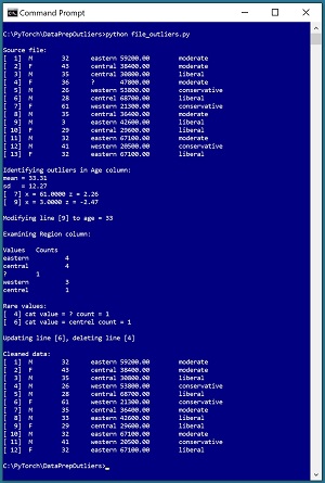 [Click on image for larger view.] Figure 1: Programmatically Dealing with Outlier Data
The demo is a Python language program that examines and performs a series of transformations on the original data. The first five lines of the demo source data are:
M   32   eastern   59200.00   moderate
F   43   central   38400.00   moderate
M   35   central   30800.00   liberal
F   36   ?         47800.00   moderate
M   26   western   53800.00   conservative
. . .
There are five tab-delimited fields: sex, age, region, annual income, and political leaning. The eventual goal of the ML system that will use the data is to create a neural network that predicts political leaning from other fields. The source data file has been standardized so that all lines have the same number of fields/columns.
The demo begins by displaying the source data file. Next the demo scans through the age column and computes a z-score value for each age. Data lines with outlier values where the z-score is less than -2.0 or greater than +2.0 are displayed. These are line [7] where age = 61 and z = +2.26, and line [9] where age = 3 and z = -2.47.
When a line with an outlier value has been identified, you can do one of three things. You can ignore the data line, you can correct the data line, or you can delete the line. The demo leaves line [7] with age = 61 alone. The implication is that the person is just significantly older than the other people in the dataset. The demo updates line [9] with age = 3 by changing the age to 33. The implication is that the value was incorrectly entered and the correct age value of 33 was located in some way.
Next, the demo scans through the region column and computes a frequency count for each value. There are four instances of "eastern", four instances of "central", and three instances of "western." There is one instance of "?" in line [4] and one instance of "centrel" in line [6]. The demo deletes line [4]. The implication is that "?" was entered as a placeholder value to mean "unknown" and that the correct region value could not be determined. The demo updates line [6] by replacing "centrel" with "central." The implication is that this was a typo.
To summarize, outliers are unusual values. For numeric variables, one way to find outliers is to compute z-scores. For categorical variables, one way to find outliers is to compute frequency counts.
This article assumes you have intermediate or better skill with a C-family programming language. The demo program is coded using Python but you shouldn't have too much trouble refactoring the demo code to another language if you wish. The complete source code for the demo program is presented in this article. The source code is also available in the accompanying file download.
The Data Preparation Pipeline
Although data preparation is different for every source dataset, in general the data preparation pipeline for most ML systems is usually something similar to the steps shown in Figure 2.
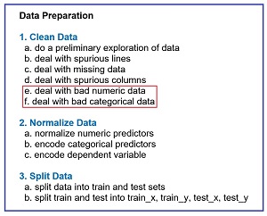 [Click on image for larger view.] Figure 2: Data Preparation Pipeline Typical Tasks
Data preparation for ML is deceptive because the process is conceptually easy. However, there are many steps, and each step is much trickier than you might expect if you're new to ML. This article explains the fifth and sixth steps in Figure 2. Future Data Science Lab articles will explain the other steps. The articles can be found here.
The tasks in Figure 2 are usually not followed strictly sequentially. You often have to backtrack and jump around to different tasks. But it's a good idea to follow the steps shown in order as much as possible. For example, it's better to deal with missing data before dealing with bad data, because after you get rid of missing data, all lines will have the same number of fields which makes it dramatically easier to compute column metrics such as the mean of a numeric field or rare occurrences in a categorical field.
The Demo Program
The structure of the demo program, with a few minor edits to save space, is shown in Listing 1. I indent my Python programs using two spaces, rather than the more common four spaces or a tab character, as a matter of personal preference. The program has six worker functions plus a main() function to control program flow. The purpose of worker functions line_count(), show_file(), delete_lines(), show_numeric_outliers(), show_cat_outliers(), and update_line() should be clear from their names.
Listing 1: Outlier Data Detection Demo Program
# file_outliers.py
# Python 3.7.6  NumPy 1.18.1

import numpy as np

def line_count(fn): . . .

def show_file(fn, start, end, indices=False,
 strip_nl=False): . . .

def delete_lines(src, dest, omit_lines): . . .

def show_numeric_outliers(fn, col, z_max,
  delim): . . .

def show_cat_outliers(fn, col, ct_min,
  delim): . . .

def update_line(src, dest, line_num, col_num,
  new_val, delim): . . .

def main():
  # 1. display source file
  print("\nSource file: ")
  fn = ".\\people_no_missing.txt"
  show_file(fn, 1, 999, indices=True, strip_nl=True)

  # 2. numeric outliers
  print("\nIdentifying outliers in Age column:")
  fn = ".\\people_no_missing.txt"
  show_numeric_outliers(fn, 2, 2.0, "\t")  # age

  print("\nModifying line [9] to age = 33")
  src = ".\\people_no_missing.txt"
  dest = ".\\people_no_missing_update1.txt"
  update_line(src, dest, 9, 2, "33", "\t")

  # 3. categorical outliers
  print("\nExamining Region column:")
  fn = ".\\people_no_missing_update1.txt"
  show_cat_outliers(fn, 3, ct_min=1, delim="\t")

  print("\nUpdating line [6], deleting line [4]")
  src = ".\\people_no_missing_update1.txt"
  dest = ".\\people_no_missing_update2.txt"
  update_line(src, dest, 6, 3, "central", "\t")

  src = ".\\people_no_missing_update2.txt"
  dest = ".\\people_clean.txt"
  delete_lines(src, dest, [4])

  print("\nCleaned data: ")
  fn = ".\\people_clean.txt"
  show_file(fn, 1, 999, indices=True, strip_nl=True)

if __name__ == "__main__":
  main()
Program execution begins with:
def main():
  # 1. display source file
  print("\nSource file: ")
  fn = ".\\people_no_missing.txt"
  show_file(fn, 1, 999, indices=True, strip_nl=True). . .
The first step when working with any machine learning data file is to do a preliminary investigation. The source data is named people_no_missing.txt ("no missing columns") and has only 13 lines to keep the main ideas of dealing with outlier data as clear as possible. The number of lines in the file could have been determined by a call to the line_count() function. The entire data file is examined by a call to show_file() with arguments start=1 and end=999. In most cases you'll examine just specified lines of the data file rather than the entire file.
The indices=True argument instructs show_file() to display 1-based line numbers. With some data preparation tasks it's more natural to use 1-based indexing, but with other tasks it's more natural to use 0-based indexing. Either approach is OK but you've got to be careful of off-by-one errors. The strip_nl=True argument instructs function show_file() to remove trailing newlines from the data lines before printing them to the shell so that there aren't blank lines between data lines in the display.
The demo continues with:
# 2. numeric outliers
  print("\nIdentifying outliers in Age column:")
  fn = ".\\people_no_missing.txt"
  show_numeric_outliers(fn, 2, 2.0, "\t")  # age
  print("\nModifying line [9] to age = 33")
  src = ".\\people_no_missing.txt"
  dest = ".\\people_no_missing_update1.txt"
  update_line(src, dest, 9, 2, "33", "\t")
. . .
The call to function show_numeric_outliers() means, "Scan the age values in 1-based column number [2], and display lines where the z-score is less than or equal to -2.0 or greater than or equal to +2.0."
The call to function update_line() means, "Take file people_no_missing.txt, change the age value in 1-based column [2] on 1-based line number [9] to "33" and save the result as people_no_missing_update1.txt."
Function update_line() uses a functional programming paradigm and accepts a source file and writes the results to a destination file. It's possible to implement update_line() so that the source file is modified. I do not recommend this approach. It's true that using source and destination files in a data preparation pipeline creates several intermediate files. But you can always delete intermediate files when they're no longer needed. If you corrupt a data file, especially a large one, recovering your data can be very painful or in some cases, impossible.
The demo program examines only the age column. In a non-demo scenario you should examine all numeric columns. The demo continues by examining the region column of categorical values and updating line [6] from "centrel" to "central":
# 3. categorical outliers
  print("\nExamining Region column:")
  fn = ".\\people_no_missing_update1.txt"
  show_cat_outliers(fn, 3, ct_min=1, delim="\t")

  print("\nUpdating line [6], deleting line [4]")
  src = ".\\people_no_missing_update1.txt"
  dest = ".\\people_no_missing_update2.txt"
  update_line(src, dest, 6, 3, "central", "\t")
. . .
The call to function show_cat_outliers() means, "Scan the region values in 1-based column [3], and display lines where a region value occurs 1 time or less." Note that "one time or less" usually means exactly one time because there can't be any frequency counts of zero unless an external list of possible values was supplied to the show_cat_outliers() function.
The demo program concludes by deleting line [4] which has a region value of "?" and then displaying the final people_clean.txt result file:
. . .
  src = ".\\people_no_missing_update2.txt"
  dest = ".\\people_clean.txt"
  delete_lines(src, dest, [4])

  print("\nCleaned data: ")
  fn = ".\\people_clean.txt"
  show_file(fn, 1, 999, indices=True, strip_nl=True)

if __name__ == "__main__":
  main()
Notice that updating then deleting is not the same as deleting then updating. If you update, line numbering does not change but if you did a delete line [4] followed by update line [6], after the delete operation line numbering changes and so you'd update the wrong line.
Exploring the Data
When working with data for an ML system you always need to determine how many lines there are in the data, how many columns/fields there are on each line, and what type of delimiter is used. The demo defines a function line_count() as:
def line_count(fn):
  ct = 0
  fin = open(fn, "r")
  for line in fin:
    ct += 1
  fin.close()
  return ct
The file is opened for reading and then traversed using a Python for-in idiom. Each line of the file, including the terminating newline character, is stored into variable named "line" but that variable isn't used. There are many alternative approaches.
The definition of function show_file() is presented in Listing 2. As is the case with all data preparation functions, there are many possible implementations.
Listing 2: Displaying Specified Lines of a File
def show_file(fn, start, end, indices=False,
  strip_nl=False):
  fin = open(fn, "r")

  ln = 1            # advance to start line
  while ln < start:
    fin.readline()
    ln += 1

  while ln <= end:    # show specified lines
    line = fin.readline()
    if line == "": break  # EOF
    if strip_nl == True:
      line = line.strip()
    if indices == True:
      print("[%3d]  " % ln, end="")
    print(line)
    ln += 1
  fin.close()
Because the while-loop terminates with a break statement, if you specify an end parameter value that's greater than the number of lines in the source file, such as 999 for the 13-line demo data, the display will end after the last line has been printed, which is usually what you want.
Finding Numeric Outlier Data
The demo program definition of function show_numeric_outlers() is presented in Listing 3. There are several ways to identify outlier values in a numeric column. The approach I prefer is to compute a z-score value for each raw value and then examine lines where the z-score is greater than or less than a plus-or-minus problem-dependent threshold value, typically about 2.0, 3.0, or 4.0. The z-score for a numeric value x in a column of data is computed as z = (x - mean) / sd where mean is the average of all values in the column and sd is the standard deviation of all values in the column.
Suppose you have only n = 3 lines of data and one of the columns is age with values (28, 34, 46). The mean of the column is (28 + 34 + 46) / 3 = 36.0. The standard deviation is the square root of the sum of the squared difference of each value and the mean, divided by the number of values, and so is:
sd = sqrt( [(28 - 36.0)^2 + (34 - 36.0)^2 + (46 - 36.0)^2] / 3 )
     = sqrt( [(-8.0)^2 + (-2.0)^s + (10.0)^2 ] / 3 )
     = sqrt( [64.0 + 4.0 + 100.0] / 3 )
     = sqrt( 168.0 / 3 )
     = sqrt(56.0)
     = 7.48
Therefore the z-score values of the three ages are:
x = 28, z = (28 - 36.0) / 7.48 = -1.07
x = 34, z = (34 - 36.0) / 7.48 = -0.27
x = 46, z = (46 - 36.0) / 7.48 = +1.34
A z-score value that is positive corresponds to an x value that is greater than the mean value, and a z-score that is negative corresponds to an x value that is less than the mean value. For data that is normally distributed, meaning follows the Gaussian, bell-shaped distribution, almost all z-score values will be between -4.0 and +4.0 so values outside that range are usually outliers.
Listing 3: Identifying Numeric Outliers Using Z-Score Values
def show_numeric_outliers(fn, col, z_max, delim):
  # need 3 passes so read into memory
  ct = line_count(fn)
  data = np.empty(ct, dtype=np.object)

  fin = open(fn, "r")
  i = 0
  for line in fin:
    data[i] = line
    i += 1
  fin.close()

  # compute mean, sd of a 1-based col
  sum = 0.0
  for i in range(len(data)):
    line = data[i]
    tokens = line.split(delim)
    sum += np.float32(tokens[col-1])
  mean = sum / len(data)

  ss = 0.0
  for i in range(len(data)):
    line = data[i]
    tokens = line.split(delim)
    x = np.float32(tokens[col-1])
    ss += (x - mean) * (x - mean)
  sd = np.sqrt(ss / len(data))  # population sd
  print("mean = %0.2f" % mean)
  print("sd   = %0.2f" % sd)

  # display outliers
  for i in range(len(data)):
    line = data[i]
    tokens = line.split(delim)
    x = np.float32(tokens[col-1])
    z = (x - mean) /sd
    if z <= -z_max or z >= z_max:
      print("[%3d] x = %0.4f z = %0.2f" % \
        ((i+1), x, z))
The z-score calculation uses the population standard deviation (dividing sum of squares by n) rather than the sample standard deviation (dividing by n-1). Both versions of standard deviation will work for identifying outliers. A sample standard deviation calculation is usually performed in situations where you want to estimate the standard deviation of a population from which a sample was selected.
No real-life data is exactly Gaussian-normal but computing and examining z-scores is a good way to start when identifying numeric outlier values. Another approach is to bin data and then look for bins that have low counts. For example, you could bin age values into [1, 10], [11, 20], [21, 30] and so on. If you did his for the demo data you'd see that bin [1, 10] had a count of 1 due to the age of 3 in line [12] of the raw data. You can bin raw data values or z-score values.
There are many possible approaches for computing and examining z-scores. The show_numeric_outliers() demo function uses this approach:
  read all data into a NumPy array of lines
  loop each line in memory
    accumulate sum of numeric value in target col
  compute mean = sum / n
  loop each line in memory
    accumulate sum squared deviations from mean
  compute sd = ssd / n
  loop each line in memory
    compute z using mean, sd
    if z < -threshold or z > +threshold
      display line
Because the data file has to be traversed three times to compute the mean, then the sd, and then each z-score, it makes sense to initially read the entire source file into a NumPy array of string-objects:
ct = line_count(fn)
data = np.empty(ct, dtype=np.object)
fin = open(fn, "r")
i = 0
for line in fin:
  data[i] = line
  i += 1
fin.close()
One of the many minor details when doing programmatic data preparation with Python is that a NumPy array of strings has to be specified as dtype=np.object rather than dtype=np.str as you would expect.
The demo implementation of show_numeric_outliers() computes the mean and standard deviation of the target numeric column. An alternative is to read the target column into memory using the NumPy loadtxt() function with the usecols parameter and then get the mean and standard deviation using the built-in NumPy mean() and std() functions.
Finding Categorical Outlier Data
The demo program definition of function show_cat_outlers() is presented in Listing 4. There are several ways to identify outlier values in a column of categorical values. The approach I prefer is to compute the frequency counts of each value in the target column and then look for rare values, typically those that occur once or twice in the target column.
Listing 4: Finding Categorical Outliers in a Column
def show_cat_outliers(fn, col, ct_min, delim):
  # need 2 passes so read into memory
  ct = line_count(fn)
  data = np.empty(ct, dtype=np.object)

  fin = open(fn, "r")
  i = 0
  for line in fin:
    data[i] = line
    i += 1
  fin.close()

  # construct dictionary for column
  d = dict()
  for i in range(len(data)):
    line = data[i]
    tokens = line.split(delim)
    sv = tokens[col-1]  # string value
    if sv not in d:
      d[sv] = 1
    else:
      d[sv] += 1

  print("\nValues \t Counts")
  for (sv,  ct) in d.items():
    print("%s \t %d" % (sv, ct))

  print("\nRare values:")
  for i in range(len(data)):
    line = data[i]
    tokens = line.split(delim)
    sv = tokens[col-1]  # string value
    ct = d[sv]  # get count
    if ct <= ct_min:
      print("[%3d] cat value = %s \
        count = %d" % ((i+1), sv, ct))
The idea is to create a Dictionary object where the key is a categorical value like "western" and the value is a frequency count like 3. Then the specified column is traversed. If the current categorical value has not been seen before, that categorical value is added to the Dictionary with a count of 1. If the current categorical value is already in the Dictionary, the associated count is incremented.
After the Dictionary object for the specified column has been created, the collection can be traversed to show the counts of all categorical values in the column so that rare values can be identified. Additionally, the file can be traversed and lines with rare values can be displayed so that you can decided whether to delete the line, update the line, or do nothing to the line.
Updating a Line
When a line of data that has an outlier numeric or categorical value has been identified, if the outlier value is a simple error such as a typo, one possible action is to update the line. The demo program implements a function update_line() shown in Listing 5.
In pseudo-code, the approach used by the demo to update is:
  loop until reach target line of src
    read line, write to dest
  end-loop
  read line-to-update
  split line into tokens
  replace target token with new value
  reconstruct line, write to dest
  loop remaining lines
    read from src, write to dest
  end-loop
Listing 5: Updating a Line
def update_line(src, dest, line_num, col_num,
  new_val, delim):
  # line_num and col_num are 1-based
  fin = open(src, "r")
  fout = open(dest, "w")
  ln = 1

  while ln < line_num:
    line = fin.readline()  # has embedded nl
    fout.write(line)
    ln += 1

  line_to_update = fin.readline()  # trailing nl
  tokens = line_to_update.split(delim)
  tokens[col_num-1] = new_val  # 0-based

  s = ""
  for j in range(len(tokens)):  # including nl
    if j == len(tokens)-1:  # at the newline
      s += tokens[j]
    else:
      s += tokens[j] + delim  # interior column
  fout.write(s)  # must have embedded nl

  for line in fin:
    fout.write(line)  # remaining lines

  fout.close(); fin.close()
  return
As is the case with most data preparation functions, function update_line() is not conceptually difficult but there are many details to deal with, such as correctly handling the embedded trailing newline character in each line of data.
Deleting a Line
When an outlier value on a line is determined to be an uncorrectable error, in most cases the best option is to delete the line. The demo program defines a delete_lines() function that removes one or more 1-based lines from a source file and writes the result to a destination file:
def delete_lines(src, dest, omit_lines):
  fin = open(src, "r"); fout = open(dest, "w")
  line_num = 1
  for line in fin:
    if line_num in omit_lines:
      line_num += 1
    else:
      fout.write(line)  # has embedded nl
      line_num += 1
  fout.close(); fin.close()
The omit_lines parameter can be a Python list such as [1, 3, 5] or a NumPy array of integer values such as np.array([1, 3, 5], dtype=np.int64). In situations where you want to delete a single line from the source file, you should specify the line using list notation, such as [3] rather than a simple scalar such as 3.
Wrapping Up
When preparing data for use in a machine learning system, no single part of the preparation pipeline is conceptually difficult but there are many steps and each step is time consuming and error prone. The net effect is that data preparation almost always takes much longer than expected.
After the steps explained in this article have been performed, the data is clean in the sense that there are no lines with missing columns so that all lines have a standardized format, and there are no lines with erroneous outlier values. The next step is to normalize numeric values so that they're in roughly the same range, to prevent variables with large magnitudes, such as annual income, don't overwhelm variables with small magnitude, such as age. After normalizing, the data must be encoded to convert categorical values such as "central" into numeric vectors like (0, 1, 0).