The Data Science Lab
Binary Classification Using PyTorch: Preparing Data
Dr. James McCaffrey of Microsoft Research kicks off a series of four articles that present a complete end-to-end production-quality example of binary classification using a PyTorch neural network, including a full Python code sample and data files.
The goal of a binary classification problem is to predict an output value that can be one of just two possible discrete values, such as "male" or "female." This article is the first in a series of four articles that present a complete end-to-end production-quality example of binary classification using a PyTorch neural network. The example problem is to predict if a banknote (think euro or dollar bill) is authentic or a forgery based on four predictor variables extracted from a digital image of the banknote.
The process of creating a PyTorch neural network binary classifier consists of six steps:
- Prepare the training and test data
- Implement a Dataset object to serve up the data
- Design and implement a neural network
- Write code to train the network
- Write code to evaluate the model (the trained network)
- Write code to save and use the model to make predictions for new previously unseen data
Each of the six steps is fairly complicated, and the six steps are tightly coupled, which adds to the difficulty. This article covers the first two steps.
A good way to see where this series of articles is headed is to take a look at the screenshot of the demo program in Figure 1. The demo begins by creating Dataset and DataLoader objects which have been designed to work with the well-known Banknote Authentication data. Next, the demo creates a 4-(8-8)-1 deep neural network. Then the demo prepares training by setting up a loss function (binary cross entropy), a training optimizer function (stochastic gradient descent) and parameters for training (learning rate and max epochs).
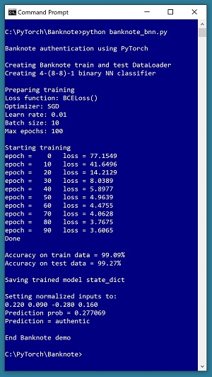 [Click on image for larger view.] Figure 1: Banknote Binary Classification in Action
The demo trains the neural network for 100 epochs. An epoch is one complete pass through the training data. For example, if there were 2,000 training data items and training was performed using batches of 50 items at a time, one epoch would consist processing 40 batches of data. During training, the demo computes and displays a measure of the current error. Because error slowly decreases, training is succeeding.
After training the network, the demo program computes the classification accuracy of the model on the training data (99.09 percent correct) and on the test data (99.27 percent correct). Because the two accuracy values are similar, it is likely that model overfitting has not occurred. After evaluating the trained model, the demo program saves the model using the state dictionary approach, which is the most common of three standard techniques.
The demo concludes by using the trained model to make a prediction. The four normalized input predictor values are (0.22, 0.09, -0.28, 0.16). The computed output value is 0.277069 which is less than 0.5 and therefore the prediction is class 0, which in turn means authentic banknote.
This article assumes you have an intermediate or better familiarity with a C-family programming language, preferably Python, but doesn't assume you know very much about PyTorch. The complete source code for the demo program, and the two data files used, are available in the download that accompanies this article. All normal error checking code has been omitted to keep the main ideas as clear as possible.
To run the demo program, you must have Python and PyTorch installed on your machine. The demo programs were developed on Windows 10 using the Anaconda 2020.02 64-bit distribution (which contains Python 3.7.6) and PyTorch version 1.6.0 for CPU installed via pip. You can find detailed step-by-step installation instructions for this configuration in my blog post "Installing PyTorch 1.5 for CPU on Windows 10 with Anaconda 2020.02 for Python 3.7."
The Banknote Authentication Data
The raw Banknote Authentication data looks like:
3.6216, 8.6661, -2.8073, -0.44699, 0
4.5459, 8.1674, -2.4586, -1.46210, 0
. . .
-2.5419, -0.65804, 2.6842, 1.1952, 1
The raw data can be found online at banknote authentication Data Set. Each line of data represents a 400 x 400 pixel image of one banknote. The first four values on each line are image variance, skewness, kurtosis and entropy. The fifth value is the class to predict, encoded as 0 for authentic and 1 for forgery. There are 1,372 data items, with 762 class 0 and 610 class 1.
Because the Banknote data has four dimensions, it's not possible to easily display the data in a graph. But you can get a good idea of what the data is like by examining the graph in Figure 2. It shows an 80-item subset of the raw data, with just the kurtosis and entropy predictor variables. Notice the data is not linearly separable so simple classification techniques such as logistic regression, decision trees and non-kernel support vector machines, would likely create poor prediction models.
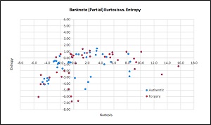 [Click on image for larger view.] Figure 2: Partial Banknote Authentication Data
To prepare the data, first I normalized the four predictor values on each line by dividing each value by 20 so that all the values are between -1.0 and +1.0. In theory, normalizing numeric predictor values isn't necessary, but in practice normalization usually leads to a model with better prediction accuracy. Instead of dividing by a constant, alternative normalization techniques include min-max normalization and z-score normalization.
Because the raw data has no categorical predictor variables, there was no need for encoding. For example, if there was a predictor variable "color" with possible values blue, green, or yellow, I would have encoded blue = (1, 0, 0), green = (0, 1, 0), yellow = (0, 0, 1).
After normalizing the raw data, I replaced the original comma delimiter characters with tab characters, just as a matter of personal preference. Next, I added 1-based ID numbers from 0001 to 1372. After normalizing, changing delimiters and adding ID values, the 1,372 items look like:
0001  0.181080  0.433305  -0.140365  -0.022350  0
0002  0.227295  0.408370  -0.122930  -0.073105  0
. . .
1372 -0.127095 -0.032902   0.134210   0.059760  1
Then using a utility script, I split the normalized data file into a training data file with 1,097 randomly selected items (80 percent of the 1,372 items) and a test data file with 275 items (the other 20 percent). The ID numbers can be used to identify which items went to the training file and which went to the test file.
The Overall Program Structure
The overall structure of the demo PyTorch binary classification program, with a few minor edits to save space, is shown in Listing 1. I indent my Python programs using two spaces rather than the more common four spaces as a matter of personal preference.
Listing 1: The Structure of the Demo Program
# banknote_bnn.py
# PyTorch 1.6.0-CPU Anaconda3-2020.02
# Python 3.7.6 Windows 10

import numpy as np
import torch as T
device = T.device("cpu")

# IDs 0001 to 1372 added
# data has been k=20 normalized (all four columns)
# ID  variance  skewness  kurtosis  entropy  class
# [0]    [1]      [2]       [3]       [4]     [5]
#  (0 = authentic, 1 = forgery)  # verified
# train: 1097 items (80%), test: 275 item (20%)

class BanknoteDataset(T.utils.data.Dataset):
  def __init__(self, src_file, num_rows=None):
  def __len__(self): . . .
  def __getitem__(self, idx): . . .

# ----------------------------------------------------

def accuracy(model, ds): . . .

# ----------------------------------------------------

class Net(T.nn.Module):
  def __init__(self): . . .
  def forward(self, x):

# ----------------------------------------------------

def main():
  # 0. get started
  print("Banknote authentication using PyTorch ")
  T.manual_seed(1)
  np.random.seed(1)

  # 1. create Dataset and DataLoader objects
  # 2. create neural network
  # 3. train network
  # 4. evaluate model
  # 5. save model
  # 6. make a prediction
  print("End Banknote demo ")

if __name__== "__main__":
  main()
It's important to document the versions of Python and PyTorch being used because both systems are under continuous development. Dealing with versioning incompatibilities is a significant headache when working with PyTorch and is something you should not underestimate.
I prefer to use "T" as the top-level alias for the torch package. Most of my colleagues don't use a top-level alias and spell out "torch" dozens of times per program. Also, I use the full form of sub-packages rather than supplying aliases such as "import torch.nn.functional as functional." In my opinion, using the full form is easier to understand and less error-prone than using many aliases.
The demo program defines a program-scope CPU device object. I usually develop my PyTorch programs on a desktop CPU machine. After I get that version working, converting to a CUDA GPU system only requires changing the global device object to T.device("cuda") plus a minor amount of debugging.
The demo program defines just one helper method, accuracy(). All of the rest of the program control logic is contained in a main() function. It is possible to define other helper functions such as train_net(), evaluate_model() and save_model(), but in my opinion this modularization approach makes the program more difficult to understand rather than easier to understand.
Defining a Banknote Dataset Class
Serving up batches of data for training a network and evaluating the accuracy of a trained model is a bit trickier than you might expect if you're new to PyTorch. In the early days of PyTorch, the most common approach was to write completely custom code. You can still write one-off code for loading data, but now the most common approach is to implement a Dataset and DataLoader. Briefly, a Dataset object loads all training or test data into memory, and a DataLoader object serves up the data in batches.
You can think of a PyTorch Dataset as an interface that must be implemented. At a minimum, you must define an __init__() method which reads data from file into memory, a __len__() method which returns the total number of items in the source data, and a __getitem__() method which returns a single batch of data items. There are many design alternatives and no two Dataset class definitions will be the same.
A DataLoader object is instantiated by passing in a Dataset object. The DataLoader object can be iterated, serving up one batch of data at a time. Unlike the Dataset, a DataLoader is ready to use as-is.
The definition of class BanknoteDataset is shown in
Listing 2. In most cases, the structures of the training and test data files are the same and you can use a single Dataset definition for both files. If the structures of your files are different, then you'd have to define two different Dataset classes, or parameterize the Dataset definition.
Listing 2: Class BanknoteDataset Definition
class BanknoteDataset(T.utils.data.Dataset):

  def __init__(self, src_file, num_rows=None):
    all_data = np.loadtxt(src_file, max_rows=num_rows,
      usecols=range(1,6), delimiter="\t", skiprows=0,
      dtype=np.float32)  # strip IDs off

    self.x_data = T.tensor(all_data[:,0:4],
      dtype=T.float32).to(device)
    self.y_data = T.tensor(all_data[:,4],
      dtype=T.float32).to(device)
    self.y_data = self.y_data.reshape(-1,1)

  def __len__(self):
    return len(self.x_data)

  def __getitem__(self, idx):
    if T.is_tensor(idx):
      idx = idx.tolist()
    preds = self.x_data[idx,:]  # idx rows, all 4 cols
    lbl = self.y_data[idx,:]    # idx rows, the 1 col
    sample = { 'predictors' : preds, 'target' : lbl }
    return sample
The __init__() method begins by reading all relevant data from file into memory using the NumPy loadtxt() function:
def __init__(self, src_file, num_rows=None):
  all_data = np.loadtxt(src_file, max_rows=num_rows,
    usecols=range(1,6), delimiter="\t", skiprows=0,
    dtype=np.float32)  # strip IDs off
The Banknote data stores both predictor values and labels-to-predict values in the same file, so both can be read at the same time. A slightly less efficient alternative is to read the predictor values with one call to loadtxt() and then read the values-to-predict with a second call.
Python has dozens of ways to read a text file into memory, but using loadtxt() is my technique of choice. Some of my colleagues prefer using the NumPy genfromtxt() or fromfile() functions, or the Pandas read_csv() function.
Notice that the demo program call to loadtxt() reads columns 1 to 5 into memory, so the ID values in column 0 are not used. Therefore, matrix all_data has the four predictor values in columns [0] through [3], and the 0-or-1 values to predict in column [4]. Off-by-one errors are common but minor annoyances when reading data.
The data is read into a NumPy matrix as float32 values. During training, the binary classification loss function is expecting a single 0.0 or 1.0 floating point value rather than a 0 or 1 integer value. This is an example of what I mean by the PyTorch components being tightly coupled. The consequence is that it's rarely possible to develop a PyTorch program in a strictly sequential manner -- it's often necessary for you to make an assumption such as a particular data type or matrix shape, and then have to backtrack when that assumption is incorrect.
After all the data has been read into memory, the predictor rows are extracted and then converted to PyTorch tensors:
self.x_data = T.tensor(all_data[:,0:4],
  dtype=T.float32).to(device)
The "[:,0:4]" syntax means "all rows, columns 0 to 3 inclusive." Another chance for an off-by-one error. Many of the examples I've seen convert the input data to PyTorch tensors in the __getitem__() method rather than in the __init__() method. Because conversion to tensors is a relatively expensive operation, it's usually better to convert the data once in __init__() rather than repeatedly in the __getitem__() method.
At this point in the program execution, self.x_data is a 2-dimensional matrix with four columns. In practice, you usually need to experiment a bit and examine objects with code like:
print("x_data is ")
print(self.x_data)
print(self.x_data.shape)
input()  # pause execution
Alternatively, if you're using a powerful IDE such as Visual Studio to write your code, you can set an execution breakpoint and examine variables.
Storing the dependent target values is similar to storing the predictor values, but with one important difference:
self.y_data = T.tensor(all_data[:,4],
  dtype=T.float32).to(device)

self.y_data = self.y_data.reshape(-1,1)
The "[:,4]" syntax means "all rows, just column [4]." Because only one column is being extracted, the y_data object is a 1-dimensional vector. As it turns out, the computed output of the neural network will be a 2-dimensional column vector. To make the dimensions of the target values and the computed output values the same, you can either change the computed output to a 1-dimensional vector using the reshape() or squeeze() function, or you can expand the target vector to a 2-dimensional matrix using the reshape() function. I've seen both techniques used, but I prefer to expand the target vector to a matrix.
The statement self.y_data = self.y_data.reshape(-1,1) is a quirky Python idiom. The -1 argument to reshape() loosely means, "computer, you figure it out." For example, if y_data is a 1-dimensional vector with 10 values, then y_data.reshape(-1,1) is a 2-dimensional matrix with 1 column and so the number of rows must be 10. The same result could be obtained by the expression y_data.reshape(10,1) which is clearer in my opinion. Therefore, the demo program code can be written as:
n_vals = len(self.y_data)
self.y_data = self.y_data.reshape(n_vals,1)
The -1 argument to reshape() is useful when the shape of a vector or matrix is dynamic, but the syntax is often used even when there's no compelling need for it (which is why I present it in the demo).
The implementation of the __len__() method is simple:
def __len__(self):
  return len(self.x_data)
The Dataset object needs to be able to return the number of items it has so that the DataLoader object that uses the Dataset can determine when all data items have been processed once, and then start a new epoch. The Dataset num_rows parameter is passed to the loadtxt() max_rows parameter. If max_rows has value None, then loadtxt() will load all lines of the source data file. So, if you omit the num_rows parameter when instantiating a Dataset object, the default parameter value of None will be used, which will be passed to loadtxt() and all lines of data will be read into memory. Therefore, the __len__() method needs to return len(self.x_data), the actual number of lines of data read, rather than num_rows, which could be None. The moral of this story is that even simple-looking PyTorch statements must be thought through very carefully.
The __getitem__() method is defined as:
def __getitem__(self, idx):
  if T.is_tensor(idx):
    idx = idx.tolist()
  preds = self.x_data[idx,:]  # idx rows, all 4 cols
  lbl = self.y_data[idx,:]    # idx rows, the 1 col
  sample = { 'predictors' : preds, 'target' : lbl }
  return sample
The method returns one or more data items as a Dictionary object where a key of "predictors" gives the predictor x values and a key of "target" gives the 0-or-1 target values. It is common practice to name the parameter indicating which items to return as "idx," but that name is slightly misleading because in most cases idx is a Python list object such as [0, 2, 5], meaning rows [0], [2] and [5] are fetched. So, idx might better be named "indices" or "list_of_indices."
The method begins by checking the idx parameter to see if it is a PyTorch tensor and if so, converts the the tensor to an ordinary list. You can omit this check if you're sure that a tensor will never be passed to the __getitem__() method. The return Dictionary value is created and populated in a single statement which might be a bit confusing if you're relatively new to Python. The demo code can be written in a less-terse fashion as:
sample = dict()   # or sample = {}
sample["predictors"] = preds
sample["target"] = lbl
When writing PyTorch programs, there's always a tradeoff between short but sometimes difficult-to-read code, and clearer but longer code. Notice that the "predictors" and "target" keys are magic strings in a sense and contribute to the tight coupling of the system. Alternative designs include defining the keys as global program-scope variables at the beginning of the program, or parameterizing the key names as strings.
Testing the Dataset
It's good practice to test a Dataset and DataLoader before trying to use them to train a neural network. The short program in Listing 3 shows an example. The test program sets up a Dataset with just the first five items from the 1,097 normalized Banknote training items. Then the tester iterates two times through the five items, in batches of size two items. Therefore, each epoch serves up batches of 2, 2 and 1 items. See the screenshot in Figure 3.
Listing 3: Testing the Dataset using a DataLoader
# test_dataset.py

import numpy as np
import torch as T
device = T.device("cpu")

# class BanknoteDataset goes here
# see Listing #2

src = ".\\Data\\banknote_k20_train.txt"
train_ds = BanknoteDataset(src, num_rows=5)
train_ldr = T.utils.data.DataLoader(train_ds,
  batch_size=2, shuffle=True)
for epoch in range(2):
  print("\n\n Epoch = " + str(epoch))
  for (bat_idx, batch) in enumerate(train_ldr):
    print("------------------------------")
    X = batch['predictors']
    Y = batch['target']
    print("bat_idx = " + str(bat_idx))
    print(X)
    print(Y)

print("End test ")
The test program assumes the data files are in a sub-directory named Data. The PyTorch DataLoader class is defined in the torch.utils.data module. A DataLoader has 10 optional parameters, but in most situations you pass only a (required) Dataset object, a batch size (the default is 1) and a shuffle (True or False, default is False) value. The shuffle parameter controls whether the data items should be served up in random order, typically during training, or in sequential order, typically during model evaluation.
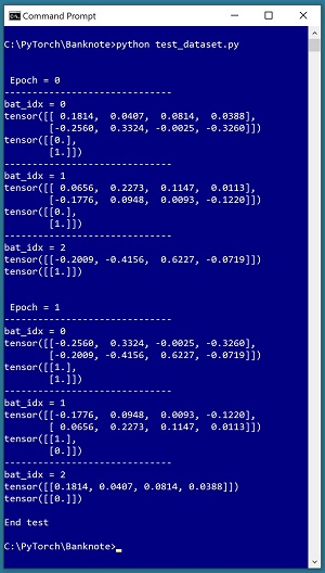 [Click on image for larger view.] Figure 3: Testing the Dataset using a DataLoader
The core statement that uses the Dataset and DataLoader is:
for (bat_idx, batch) in enumerate(train_ldr):
  . . .
The enumerate() function is a built-in Python mechanism to walk through iterable objects, which include DataLoader objects. The return value is a tuple where the first value is the 0-based batch index and the second value is a batch of data items stored as a Dictionary object. The short test program is just a beginning and you should test any Dataset object you define by iterating through all data items, with both the training and test data, and with the shuffle parameter set to both True and False.
Wrapping Up
The demo code presented in this article assumes that the neural binary classifier has a single output node with a value between 0.0 and 1.0 where a computed output value less than 0.5 corresponds to a prediction of class 0, and a computed output value greater than 0.5 corresponds to class 1. This is by far the most common scheme used for neural binary classification. But there are other designs. For example, it is possible to design a binary classifier with two output nodes where a target output of (1, 0) represents class 0, and a target of (0, 1) represents class 1. For most alternative binary classifier architectures, you would have to use a Dataset definition that more closely resembles one designed for multi-class classification than for binary classification.
The example code presented in this article can be used as a template for most binary classification problems. One exception is a scenario where your training data is too large to fit entirely into memory. Fortunately these situations are relatively rare. For huge data files, the most usual approach is to define a Dataset object where the __init__() method reads part of the huge file into a buffer, and then when all of the buffer data has been process by calls to the __getitem__() method, a program-defined reload() method fills the buffer with the next block of data.