The Data Science Lab
Wasserstein Distance Using C# and Python
Dr. James McCaffrey of Microsoft Research shows how to compute the Wasserstein distance and explains why it is often preferable to alternative distance functions, used to measure the distance between two probability distributions in machine learning projects.
A common task in machine learning is measuring the distance between two probability distributions. For example, suppose distribution P = (0.2, 0.5, 0.3) and distribution Q = (0.1, 0.8, 0.1). What is the distance between P and Q? The distance between two distributions can be used in several ways, including measuring the difference between two images, comparing a data sample to the population from which the sample was drawn, and measuring loss/error for distribution-based neural systems such as variational autoencoders (VAEs).
There are many different ways to measure the distance between two probability distributions. Some of the most commonly used distance functions are Kullback-Leibler divergence, symmetric Kullback-Leibler distance, Jensen-Shannon distance, and Hellinger distance. This article shows you how to compute the Wasserstein distance and explains why it is often preferable to alternative distance functions.
A good way to see where this article is headed is to take a look at the screenshot of a demo program in Figure 1. The demo program sets up a P distribution = (0.6, 0.1, 0.1, 0.1, 0.1) and a Q1 distribution = (0.1, 0.1, 0.6, 0.1, 0.1) and a Q2 distribution = (0.1, 0.1, 0.1, 0.1, 0.6). The graphs of the three distributions, and common sense, tell you that P is closer to Q1 than it is to Q2. The Wasserstein distance between (P, Q1) = 1.00 and Wasserstein(P, Q2) = 2.00 -- which is reasonable. However, the symmetric Kullback-Leibler distance between (P, Q1) and the distance between (P, Q2) are both 1.79 -- which doesn't make much sense.
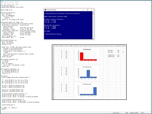 [Click on image for larger view.] Figure 1: Wasserstein Distance Demo.
This article assumes you have an intermediate or better familiarity with a C-family programming language. The demo program is implemented using Python. I also present a C# language version. The complete source code for the demo program is presented in this article and is also available in the accompanying file download. All normal error checking has been removed to keep the main ideas as clear as possible.
To run the demo program, you must have Python installed on your machine. The demo program was developed on Windows 10 using the Anaconda 2020.02 64-bit distribution (which contains Python 3.7.6). The demo program has no significant dependencies so any relatively recent version of Python 3 will work fine.
Understanding the Wasserstein Distance
The Wasserstein distance (also known as Earth Mover Distance) is best explained by an example. Suppose P = (0.2, 0.1, 0.0, 0.0, 0.3, 0.4) and Q = (0.0, 0.5, 0.3, 0.0, 0.2, 0.0, 0.0). See Figure 2. If you think of distribution P as piles of dirt and distribution Q as holes, the Wasserstein distance is the minimum amount of work required to transfer all the dirt in P to the holes in Q.
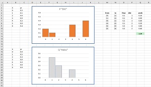 [Click on image for larger view.] Figure 2: Wasserstein Calculation Example.
The transfer can be accomplished in six steps.
- all 0.2 in dirt[0] is moved to holes[1], using up dirt[0], with holes[1] needing 0.3 more.
- all 0.1 in dirt[1] is moved to holes[1], using up dirt[1], with holes[1] needing 0.2 more.
- just 0.2 in dirt[4] is moved to holes[1], filling dirt[1], leaving 0.1 left in dirt[4].
- all remaining 0.1 in dirt[4] is moved to holes[2], using up dirt[4], with holes[2] needing 0.2 more.
- just 0.2 in dirt[6] is moved to holes[2], filling holes[2], leaving 0.2 left in dirt[6].
- all remaining 0.2 in dirt[6] is moved to holes[4], using up dirt[6], filling holes[4].
In each transfer, the amount of work done is the flow (amount of dirt moved) times the distance. The Wasserstein distance is the total amount of work done. Put slightly differently, the Wasserstein distance between two distributions is the effort required to transform one distribution into the other.
The Kullback-Leibler Divergence
A common alternative distance function is the Kullback-Leibler (KL) divergence, and a slightly improved variation called symmetric Kullback-Leibler distance. Suppose distribution P = (0.2, 0.5, 0.3) and distribution Q = (0.1, 0.3, 0.7). The Kullback-Leibler divergence is computed as the sum of the p[i] times the log(p[i] / q[i]):
KL = (0.2 * log(0.2 / 0.1)) +
     (0.5 * log(0.5 / 0.3)) +
     (0.3 * log(0.3 / 0.7))
   = (0.2 * 0.69) + (0.5 * 0.51) + (0.3 * -0.85)
   = 0.14 + 0.25 - 0.25
   = 0.14
Kullback-Leibler divergence can be implemented using Python like this:
import numpy as np
def kullback_leibler(p, q):
  n = len(p)
  sum = 0.0
  for i in range(n):
    sum += p[i] * np.log(p[i] / q[i])
  return sum
Because of the division operation in the calculation, the Kullback-Leibler divergence is not symmetric, meaning KL(P, Q) != KL(Q, P) in general. The simplest solution to this problem is to define a symmetric Kullback-Leibler distance function as KLsym(P, Q) = KL(P, Q) + KL(Q, P). However, Kullback-Leibler still has the problem that if any of the values in the P or Q distributions are 0, you run into a division-by-zero problem. One way to deal with this is to add a tiny value, such as 1.0e-5, to all distribution values, but this has the feel of a hack. In short, the common Kullback-Leibler distance function has conceptual and engineering problems.
Implementing Wasserstein Distance
There are many different variations of Wasserstein distance. There are versions for discrete distributions and for mathematically continuous distributions. There are versions where each data point is a single value such as 0.3 and there are versions where each data point is multi-valued, such as (0.4, 0.8). There are mathematical abstract generalizations called 2-Wasserstein, 3-Wasserstein, and so on. The version of Wasserstein distance presented in this article is for two discrete 1D probability distributions and is the 1-Wasserstein version.
The demo defines a my_wasserstein() function as:
def my_wasserstein(p, q):
  dirt = np.copy(p)
  holes = np.copy(q)
  tot_work = 0.0

  while True:  # TODO: add sanity counter check
    from_idx = first_nonzero(dirt)
    to_idx = first_nonzero(holes)
    if from_idx == -1 or to_idx == -1:
      break
    work = move_dirt(dirt, from_idx, holes, to_idx)
    tot_work += work
  return tot_work
Most of the algorithmic work is done by helper functions first_nonzero() and move_dirt(). In words, the function finds the first available dirt, then finds the first non-filled hole, then moves as much dirt as possible to the hole, and returns the amount of work done. The amount of work done on each transfer is accumulated.
Helper function first_nonzero() is simple:
def first_nonzero(vec):
  dim = len(vec)
  for i in range(dim):
    if vec[i] > 0.0:
      return i
  return -1  # no empty cells found
Helper function move_dirt() is defined as:
def move_dirt(dirt, di, holes, hi):
  if dirt[di] <= holes[hi]:   # use all dirt
    flow = dirt[di]
    dirt[di] = 0.0            # all dirt got moved
    holes[hi] -= flow         # less to fill now
  elif dirt[di] > holes[hi]:  # use just part of dirt
    flow = holes[hi]          # fill remainder of hole
    dirt[di] -= flow          # less dirt left
    holes[hi] = 0.0           # hole is filled
  dist = np.abs(di - hi)
  return flow * dist          # work
The condition dirt[di] <= holes[hi] means the amount of available dirt at [di] is not enough to fill the hole at [hi]. Therefore, all available dirt at [di] is moved. The condition dirt[di] > holes[hi] means the current dirt at [di] is more than there is room for in the holes at [hi] so only part of the dirt is used.
The Complete Demo Program
The complete Python version of the demo program is presented in Listing 1. The demo program defines separate helpers first_nonzero() and move_dirt(), and the calling my_wasserstein() function. An alternative structure is to wrap the three functions in a class. Another design alternative is to define first_nonzero() and move_dirt() as nested local functions inside the my_wasserstein() function.
Listing 1: Python Version of Wasserstein Distance
# wasserstein_demo.py
# Wasserstein distance from scratch

import numpy as np

def first_nonzero(vec):
  dim = len(vec)
  for i in range(dim):
    if vec[i] > 0.0:
      return i
  return -1  # no empty cells found

def move_dirt(dirt, di, holes, hi):
  # move as much dirt at [di] as possible to h[hi]
  if dirt[di] <= holes[hi]:   # use all dirt
    flow = dirt[di]
    dirt[di] = 0.0            # all dirt got moved
    holes[hi] -= flow         # less to fill now
  elif dirt[di] > holes[hi]:  # use just part of dirt
    flow = holes[hi]          # fill remainder of hole
    dirt[di] -= flow          # less dirt left
    holes[hi] = 0.0           # hole is filled
  dist = np.abs(di - hi)
  return flow * dist          # work

def my_wasserstein(p, q):
  dirt = np.copy(p)
  holes = np.copy(q)
  tot_work = 0.0

  while True:  # TODO: add sanity counter check
    from_idx = first_nonzero(dirt)
    to_idx = first_nonzero(holes)
    if from_idx == -1 or to_idx == -1:
      break
    work = move_dirt(dirt, from_idx, holes, to_idx)
    tot_work += work
  return tot_work

def kullback_leibler(p, q):
  n = len(p)
  sum = 0.0
  for i in range(n):
    sum += p[i] * np.log(p[i] / q[i])
  return sum

def symmetric_kullback(p, q):
  a = kullback_leibler(p, q)
  b = kullback_leibler(q, p)
  return a + b

def main():
  print("\nBegin Wasserstein distance demo ")

  P =  np.array([0.6, 0.1, 0.1, 0.1, 0.1])
  Q1 = np.array([0.1, 0.1, 0.6, 0.1, 0.1])
  Q2 = np.array([0.1, 0.1, 0.1, 0.1, 0.6])

  kl_p_q1 = symmetric_kullback(P, Q1)
  kl_p_q2 = symmetric_kullback(P, Q2)

  wass_p_q1 = my_wasserstein(P, Q1)
  wass_p_q2 = my_wasserstein(P, Q2)

  print("\nKullback-Leibler distances: ")
  print("P to Q1 : %0.4f " % kl_p_q1)
  print("P to Q2 : %0.4f " % kl_p_q2)

  print("\nWasserstein distances: ")
  print("P to Q1 : %0.4f " % wass_p_q1)
  print("P to Q2 : %0.4f " % wass_p_q2)

  print("\nEnd demo ")

if __name__ == "__main__":
  main()
Because the Python language version of the demo program doesn't use any exotic libraries, it's easy to refactor the code to C# or any other c-family language. A C# version of the Wasserstein distance function is presented in Listing 2.
Listing 2: C# Version of Wasserstein Distance
using System;
namespace Wasserstein
{
  class Program
  {
    static void Main(string[] args)
    {
      Console.WriteLine("\nBegin demo \n");

      double[] P = new double[]
        { 0.6, 0.1, 0.1, 0.1, 0.1 };
      double[] Q1 = new double[]
        { 0.1, 0.1, 0.6, 0.1, 0.1 };
      double[] Q2 = new double[]
        { 0.1, 0.1, 0.1, 0.1, 0.6 };

      double wass_p_q1 = MyWasserstein(P, Q1);
      double wass_p_q2 = MyWasserstein(P, Q2);

      Console.WriteLine("Wasserstein(P, Q1) = " +
        wass_p_q1.ToString("F4"));
      Console.WriteLine("Wasserstein(P, Q2) = " +
        wass_p_q2.ToString("F4"));

      Console.WriteLine("\nEnd demo ");
      Console.ReadLine();
    }  // Main

    static int FirstNonZero(double[] vec)
    {
      int dim = vec.Length;
      for (int i = 0; i < dim; ++i)
        if (vec[i] > 0.0)
          return i;
      return -1;
    }

    static double MoveDirt(double[] dirt, int di,
      double[] holes, int hi)
    {
      double flow = 0.0;
      int dist = 0;
      if (dirt[di] <= holes[hi])
      {
        flow = dirt[di];
        dirt[di] = 0.0;
        holes[hi] -= flow;
      }
      else if (dirt[di] > holes[hi])
      {
        flow = holes[hi];
        dirt[di] -= flow;
        holes[hi] = 0.0;
      }
      dist = Math.Abs(di - hi);
      return flow * dist;
    }

    static double MyWasserstein(double[] p, double[] q)
    {
      double[] dirt = (double[])p.Clone();
      double[] holes = (double[])q.Clone();
      double totalWork = 0.0;
      while (true)
      {
        int fromIdx = FirstNonZero(dirt);
        int toIdx = FirstNonZero(holes);
        if (fromIdx == -1 || toIdx == -1)
          break;
        double work = MoveDirt(dirt, fromIdx,
          holes, toIdx);
        totalWork += work;
      }
      return totalWork;
    }
  }  // Program
}  // ns
In a production environment you'd probably want to add error checking. For example, you should check that the P and Q distributions have the same length, the values in both sum to 1.0, and so on.
Wrapping Up
In informal usage, the term "metric" means any kind of numerical measurement. But in the context of measuring the distance between two distributions the term "metric" describes a distance function that has three nice mathematical characteristics:
- if p = q, then dist(p, q) = 0 and if dist(p, q) = 0 then p = q. [identity]
- dist(p, q) = dist(q, p). [symmetry]
- dist(p, q) <= dist(p, r) + dist(r, q). [triangle inequality]
The Wasserstein distance function satisfies all three conditions and so it is a formal distance metric. Many common distance functions do not meet one or more of these conditions. For example, Kullback-Leibler divergence meets only condition 1. Symmetric Kullback-Leibler distance meets conditions 1 and 2 but not 3.
Variations of the Wasserstein distance function are used in several machine learning scenarios. For example, standard generative adversarial networks (GANs) use Kullback-Leibler divergence as a loss/error function, but WGANs (Wasserstein GANs) use the more robust Wassersein distance.
About the Author
Dr. James McCaffrey works for Microsoft Research in Redmond, Wash. He has worked on several Microsoft products including Azure and Bing. James can be reached at [email protected].